

environment and excrete waste products and waste heat. Similarly, entire ecosystems channel materials and energy through their systems. The constant influx of
“reactants” and energy into these systems and the constant removal of waste
materials and heat make it possible for these systems to function. They are clearly
open and not in equilibrium with their surroundings.
Change the values for A and B, and rerun the model for alternative initial
conditions. Can you find the steady-state conditions? How does the limit cycle
change? How are the results affected by the choice of DT and integration methods.
Once you explored the dynamics of this system and familiarized yourself
sufficiently with the models of chemical processes discussed in this part of the
book, move on to learn more about the application of physical principles and tools
to the understanding of biological processes. This is the topic of the following
chapter.
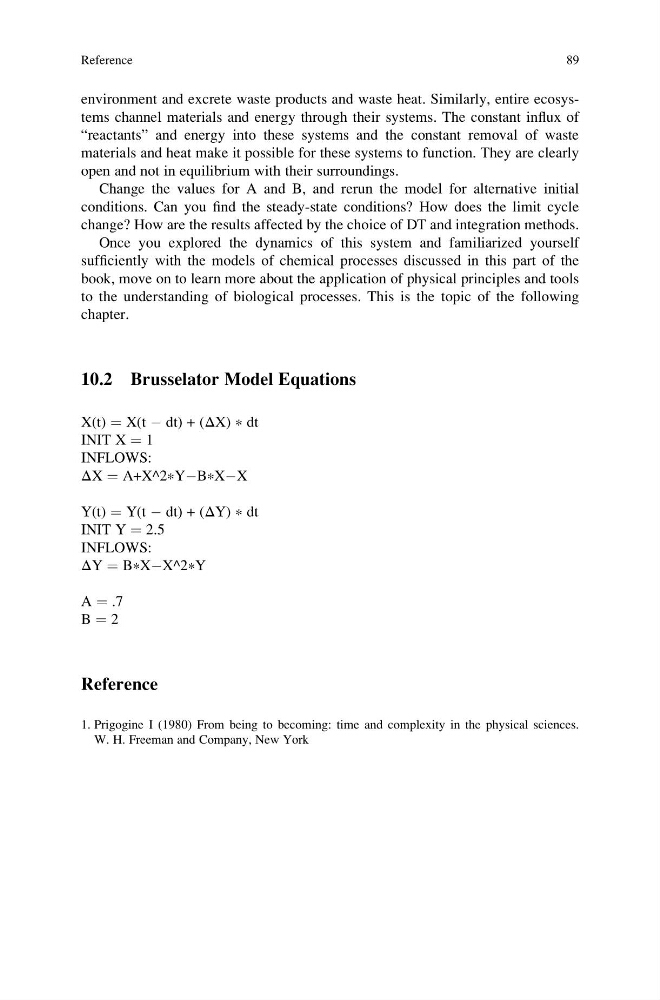
10.2 Brusselator Model Equations
X(t) ¼ X(t À dt) + (ΔX) * dt
INIT X ¼ 1
INFLOWS:
ΔX ¼ A+X^2 * YÀB * XÀX
Y(t) ¼ Y(t À dt) + (ΔY) * dt
INIT Y ¼ 2.5
INFLOWS:
ΔY ¼ B * XÀX^2 * Y
A ¼ .7
B ¼ 2
Reference
1. Prigogine I (1980) From being to becoming: time and complexity in the physical sciences.
W. H. Freeman and Company, New York
Reference
89
“reactants” and energy into these systems and the constant removal of waste
materials and heat make it possible for these systems to function. They are clearly
open and not in equilibrium with their surroundings.
Change the values for A and B, and rerun the model for alternative initial
conditions. Can you find the steady-state conditions? How does the limit cycle
change? How are the results affected by the choice of DT and integration methods.
Once you explored the dynamics of this system and familiarized yourself
sufficiently with the models of chemical processes discussed in this part of the
book, move on to learn more about the application of physical principles and tools
to the understanding of biological processes. This is the topic of the following
chapter.
10.2 Brusselator Model Equations
X(t) ¼ X(t À dt) + (ΔX) * dt
INIT X ¼ 1
INFLOWS:
ΔX ¼ A+X^2 * YÀB * XÀX
Y(t) ¼ Y(t À dt) + (ΔY) * dt
INIT Y ¼ 2.5
INFLOWS:
ΔY ¼ B * XÀX^2 * Y
A ¼ .7
B ¼ 2
Reference
1. Prigogine I (1980) From being to becoming: time and complexity in the physical sciences.
W. H. Freeman and Company, New York
Reference
89