

300
Hugh Possingham, Ian Ball, and Sandy Andelman
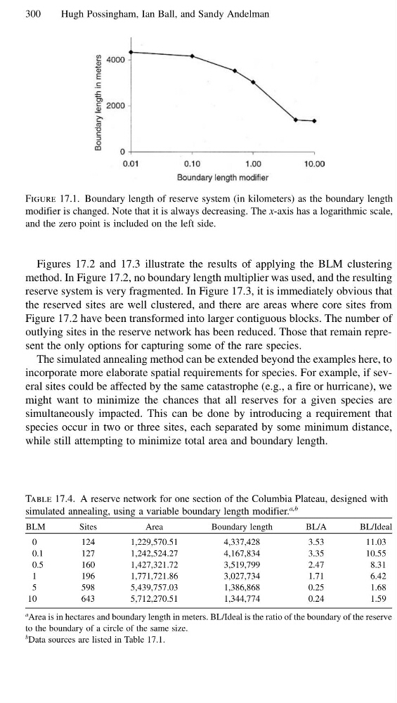
Figure 17.1. Boundary length of reserve system (in kilometers) as the boundary length
modifier is changed. Note that it is always decreasing. The x-axis has a logarithmic scale,
and the zero point is included on the left side.
Figures 17.2 and 17.3 illustrate the results of applying the BLM clustering
method. In Figure 17.2, no boundary length multiplier was used, and the resulting
reserve system is very fragmented. In Figure 17.3, it is immediately obvious that
the reserved sites are well clustered, and there are areas where core sites from
Figure 17.2 have been transformed into larger contiguous blocks. The number of
outlying sites in the reserve network has been reduced. Those that remain represent the only options for capturing some of the rare species.
The simulated annealing method can be extended beyond the examples here, to
incorporate more elaborate spatial requirements for species. For example, if several sites could be affected by the same catastrophe (e.g., a fire or hurricane), we
might want to minimize the chances that all reserves for a given species are
simultaneously impacted. This can be done by introducing a requirement that
species occur in two or three sites, each separated by some minimum distance,
while still attempting to minimize total area and boundary length.
Table 17.4. A reserve network for one section of the Columbia Plateau, designed with
simulated annealing, using a variable boundary length modifier.
a,b
BLM
Sites
Area
Boundary length
BL/A
BL/Ideal
0
124
1,229,570.51
4,337,428
3.53
11.03
0.1
127
1,242,524.27
4,167,834
3.35
10.55
0.5
160
1,427,321.72
3,519,799
2.47
8.31
1
196
1,771,721.86
3,027,734
1.71
6.42
5
598
5,439,757.03
1,386,868
0.25
1.68
10
643
5,712,270.51
1,344,774
0.24
1.59
a
Area is in hectares and boundary length in meters. BL/Ideal is the ratio of the boundary of the reserve
to the boundary of a circle of the same size.
b
Data sources are listed in Table 17.1.
Hugh Possingham, Ian Ball, and Sandy Andelman
Figure 17.1. Boundary length of reserve system (in kilometers) as the boundary length
modifier is changed. Note that it is always decreasing. The x-axis has a logarithmic scale,
and the zero point is included on the left side.
Figures 17.2 and 17.3 illustrate the results of applying the BLM clustering
method. In Figure 17.2, no boundary length multiplier was used, and the resulting
reserve system is very fragmented. In Figure 17.3, it is immediately obvious that
the reserved sites are well clustered, and there are areas where core sites from
Figure 17.2 have been transformed into larger contiguous blocks. The number of
outlying sites in the reserve network has been reduced. Those that remain represent the only options for capturing some of the rare species.
The simulated annealing method can be extended beyond the examples here, to
incorporate more elaborate spatial requirements for species. For example, if several sites could be affected by the same catastrophe (e.g., a fire or hurricane), we
might want to minimize the chances that all reserves for a given species are
simultaneously impacted. This can be done by introducing a requirement that
species occur in two or three sites, each separated by some minimum distance,
while still attempting to minimize total area and boundary length.
Table 17.4. A reserve network for one section of the Columbia Plateau, designed with
simulated annealing, using a variable boundary length modifier.
a,b
BLM
Sites
Area
Boundary length
BL/A
BL/Ideal
0
124
1,229,570.51
4,337,428
3.53
11.03
0.1
127
1,242,524.27
4,167,834
3.35
10.55
0.5
160
1,427,321.72
3,519,799
2.47
8.31
1
196
1,771,721.86
3,027,734
1.71
6.42
5
598
5,439,757.03
1,386,868
0.25
1.68
10
643
5,712,270.51
1,344,774
0.24
1.59
a
Area is in hectares and boundary length in meters. BL/Ideal is the ratio of the boundary of the reserve
to the boundary of a circle of the same size.
b
Data sources are listed in Table 17.1.