

Model Simulation ofTemporal Variability of Suspended Matter in the North Sea
59
6 ~------------------------------------'. 6
NEAC North Sea ProJect. Sile A
u,
(cm/s)
"~-~- -~-Q-~2
- -
•
4
o
1985 1986 1987 1988 1989 1990 1991 1992 1993 1994
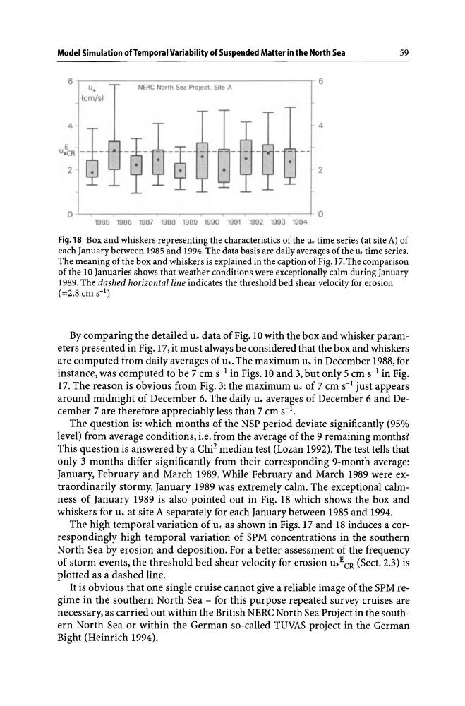
Fig.18 Box and whiskers representing the characteristics of the l4 time series (at site A) of
each January between 1985 and 1994. The data basis are daily averages of the l4 time series.
The meaning of the box and whiskers is explained in the caption of Fig. 17. The comparison
of the 10 Januaries shows that weather conditions were exceptionally calm during January
1989. The dashed horizontal line indicates the threshold bed shear velocity for erosion
(=2.8 cm S-I)
By comparing the detailed u. data of Fig. 10 with the box and whisker parameters presented in Fig. 17, it must always be considered that the box and whiskers
are computed from daily averages of u •. The maximum u. in December 1988, for
instance, was computed to be 7 cm s-1 in Figs. 10 and 3, but only 5 cm S-1 in Fig.
17. The reason is obvious from Fig. 3: the maximum u. of 7 cm s-1 just appears
around midnight of December 6. The daily u. averages of December 6 and December 7 are therefore appreciably less than 7 cm S-I.
The question is: which months of the NSP period deviate significantly (95%
level) from average conditions, i.e. from the average of the 9 remaining months?
This question is answered by a Chi 2 median test (Lozan 1992). The test tells that
only 3 months differ significantly from their corresponding 9-month average:
January, February and March 1989. While February and March 1989 were extraordinarily stormy, January 1989 was extremely calm. The exceptional calmness of January 1989 is also pointed out in Fig. 18 which shows the box and
whiskers for u. at site A separately for each January between 1985 and 1994.
The high temporal variation of u. as shown in Figs. 17 and 18 induces a correspondingly high temporal variation of SPM concentrations in the southern
North Sea by erosion and deposition. For a better assessment of the frequency
of storm events, the threshold bed shear velocity for erosion U.ECR (Sect. 2.3) is
plotted as a dashed line.
It is obvious that one single cruise cannot give a reliable image of the SPM regime in the southern North Sea - for this purpose repeated survey cruises are
necessary, as carried out within the British NERC North Sea Project in the southern North Sea or within the German so-called TUVAS project in the German
Bight (Heinrich 1994).
59
6 ~------------------------------------'. 6
NEAC North Sea ProJect. Sile A
u,
(cm/s)
"~-~- -~-Q-~2
- -
•
4
o
1985 1986 1987 1988 1989 1990 1991 1992 1993 1994
Fig.18 Box and whiskers representing the characteristics of the l4 time series (at site A) of
each January between 1985 and 1994. The data basis are daily averages of the l4 time series.
The meaning of the box and whiskers is explained in the caption of Fig. 17. The comparison
of the 10 Januaries shows that weather conditions were exceptionally calm during January
1989. The dashed horizontal line indicates the threshold bed shear velocity for erosion
(=2.8 cm S-I)
By comparing the detailed u. data of Fig. 10 with the box and whisker parameters presented in Fig. 17, it must always be considered that the box and whiskers
are computed from daily averages of u •. The maximum u. in December 1988, for
instance, was computed to be 7 cm s-1 in Figs. 10 and 3, but only 5 cm S-1 in Fig.
17. The reason is obvious from Fig. 3: the maximum u. of 7 cm s-1 just appears
around midnight of December 6. The daily u. averages of December 6 and December 7 are therefore appreciably less than 7 cm S-I.
The question is: which months of the NSP period deviate significantly (95%
level) from average conditions, i.e. from the average of the 9 remaining months?
This question is answered by a Chi 2 median test (Lozan 1992). The test tells that
only 3 months differ significantly from their corresponding 9-month average:
January, February and March 1989. While February and March 1989 were extraordinarily stormy, January 1989 was extremely calm. The exceptional calmness of January 1989 is also pointed out in Fig. 18 which shows the box and
whiskers for u. at site A separately for each January between 1985 and 1994.
The high temporal variation of u. as shown in Figs. 17 and 18 induces a correspondingly high temporal variation of SPM concentrations in the southern
North Sea by erosion and deposition. For a better assessment of the frequency
of storm events, the threshold bed shear velocity for erosion U.ECR (Sect. 2.3) is
plotted as a dashed line.
It is obvious that one single cruise cannot give a reliable image of the SPM regime in the southern North Sea - for this purpose repeated survey cruises are
necessary, as carried out within the British NERC North Sea Project in the southern North Sea or within the German so-called TUVAS project in the German
Bight (Heinrich 1994).