

Model Simulation ofTemporal Variability of Suspended Matter in the North Sea
o
SPM concentration
measured date
1 - 1.5
1.5 - 2
2 - 2.5
> 2.5
53
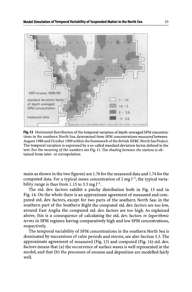
Fig.13 Horizontal distribution of the temporal variation of depth-averaged SPM concentrations in the southern North Sea, determined from SPM concentrations measured between
August 1988 and October 1989 within the framework of the British NERC North Sea Project.
The temporal variation is expressed by a so-called standard deviation factor, defined in the
text. For the meaning of the numbers see Fig. 11. The shading between the stations is obtained from inter- or extrapolation
main as shown in the two figures) are 1.76 for the measured data and 1.74 for the
computed data. For a typical mean concentration of 2 mg 1-1, the typical variability range is thus from 1.15 to 3.5 mg 1-1.
The std. dev. factors exhibit a patchy distribution both in Fig. 13 and in
Fig. 14. On the whole there is an approximate agreement of measured and computed std. dev. factors, except for two parts of the southern North Sea: in the
southern part of the Southern Bight the computed std. dev. factors are too low,
around East Anglia the computed std. dev. factors are too high. As explained
above, this is a consequence of calculating the std. dev. factors in logarithmic
terms in SPM regimes having comparatively high and low SPM concentrations,
respectively.
The temporal variability of SPM concentrations in the southern North Sea is
dominated by successions of calm periods and storms, see also Section 5.3. The
approximate agreement of measured (Fig. 13) and computed (Fig. 14) std. dev.
factors means that (a) the occurrence of surface waves is well represented in the
model, and that (b) the processes of erosion and deposition are modelled fairly
well.
o
SPM concentration
measured date
1 - 1.5
1.5 - 2
2 - 2.5
> 2.5
53
Fig.13 Horizontal distribution of the temporal variation of depth-averaged SPM concentrations in the southern North Sea, determined from SPM concentrations measured between
August 1988 and October 1989 within the framework of the British NERC North Sea Project.
The temporal variation is expressed by a so-called standard deviation factor, defined in the
text. For the meaning of the numbers see Fig. 11. The shading between the stations is obtained from inter- or extrapolation
main as shown in the two figures) are 1.76 for the measured data and 1.74 for the
computed data. For a typical mean concentration of 2 mg 1-1, the typical variability range is thus from 1.15 to 3.5 mg 1-1.
The std. dev. factors exhibit a patchy distribution both in Fig. 13 and in
Fig. 14. On the whole there is an approximate agreement of measured and computed std. dev. factors, except for two parts of the southern North Sea: in the
southern part of the Southern Bight the computed std. dev. factors are too low,
around East Anglia the computed std. dev. factors are too high. As explained
above, this is a consequence of calculating the std. dev. factors in logarithmic
terms in SPM regimes having comparatively high and low SPM concentrations,
respectively.
The temporal variability of SPM concentrations in the southern North Sea is
dominated by successions of calm periods and storms, see also Section 5.3. The
approximate agreement of measured (Fig. 13) and computed (Fig. 14) std. dev.
factors means that (a) the occurrence of surface waves is well represented in the
model, and that (b) the processes of erosion and deposition are modelled fairly
well.