

Risk, Uncertainty and Priorities - Quantitative Models
8.
'000
-
0.0 Mod'
C~I.UI, .. ~tlil .. C<- I)
'"
..
1
0,0 ltd'
449
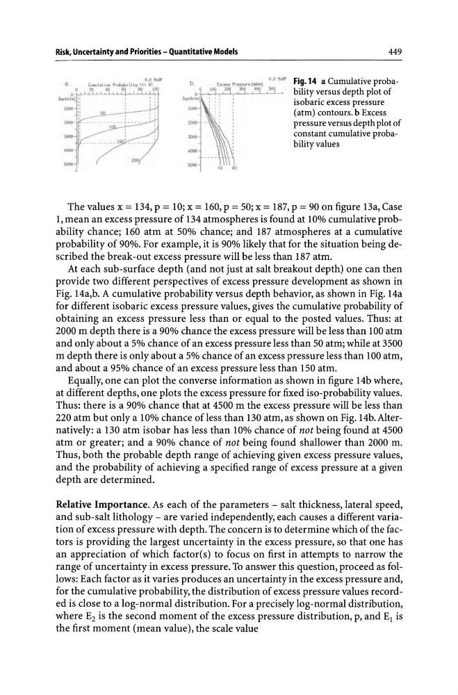
Fig.14 a Cumulative probability versus depth plot of
isobaric excess pressure
(atm) contours. b Excess
pressure versus depth plot of
constant cumulative probability values
The values x = 134, P = 10; x = 160, P = 50; x = 187, P = 90 on figure 13a, Case
1,mean an excess pressure of 134 atmospheres is found at 10% cumulative probability chance; 160 atm at 50% chance; and 187 atmospheres at a cumulative
probability of 90%. For example, it is 90% likely that for the situation being described the break-out excess pressure will be less than 187 atm.
At each sub-surface depth (and not just at salt breakout depth) one can then
provide two different perspectives of excess pressure development as shown in
Fig. 14a,b. A cumulative probability versus depth behavior, as shown in Fig. 14a
for different isobaric excess pressure values, gives the cumulative probability of
obtaining an excess pressure less than or equal to the posted values. Thus: at
2000 m depth there is a 90% chance the excess pressure will be less than 100 atm
and only about a 5% chance of an excess pressure less than 50 atm; while at 3500
m depth there is only about a 5% chance of an excess pressure less than 100 atm,
and about a 95% chance of an excess pressure less than 150 atm.
Equally, one can plot the converse information as shown in figure 14b where,
at different depths, one plots the excess pressure for fixed iso-probability values.
Thus: there is a 90% chance that at 4500 m the excess pressure will be less than
220 atm but only a 10% chance of less than 130 atm, as shown on Fig. 14b. Alternatively: a 130 atm isobar has less than lO% chance of not being found at 4500
atm or greater; and a 90% chance of not being found shallower than 2000 m.
Thus, both the probable depth range of achieving given excess pressure values,
and the probability of achieving a specified range of excess pressure at a given
depth are determined.
Relative Importance. As each of the parameters - salt thickness, lateral speed,
and sub-salt lithology - are varied independently, each causes a different variation of excess pressure with depth. The concern is to determine which of the factors is providing the largest uncertainty in the excess pressure, so that one has
an appreciation of which factor(s) to focus on first in attempts to narrow the
range of uncertainty in excess pressure. To answer this question, proceed as follows: Each factor as it varies produces an uncertainty in the excess pressure and,
for the cumulative probability, the distribution of excess pressure values recorded is close to a log-normal distribution. For a precisely log-normal distribution,
where E2 is the second moment of the excess pressure distribution, p, and E] is
the first moment (mean value), the scale value
8.
'000
-
0.0 Mod'
C~I.UI, .. ~tlil .. C<- I)
'"
..
1
0,0 ltd'
449
Fig.14 a Cumulative probability versus depth plot of
isobaric excess pressure
(atm) contours. b Excess
pressure versus depth plot of
constant cumulative probability values
The values x = 134, P = 10; x = 160, P = 50; x = 187, P = 90 on figure 13a, Case
1,mean an excess pressure of 134 atmospheres is found at 10% cumulative probability chance; 160 atm at 50% chance; and 187 atmospheres at a cumulative
probability of 90%. For example, it is 90% likely that for the situation being described the break-out excess pressure will be less than 187 atm.
At each sub-surface depth (and not just at salt breakout depth) one can then
provide two different perspectives of excess pressure development as shown in
Fig. 14a,b. A cumulative probability versus depth behavior, as shown in Fig. 14a
for different isobaric excess pressure values, gives the cumulative probability of
obtaining an excess pressure less than or equal to the posted values. Thus: at
2000 m depth there is a 90% chance the excess pressure will be less than 100 atm
and only about a 5% chance of an excess pressure less than 50 atm; while at 3500
m depth there is only about a 5% chance of an excess pressure less than 100 atm,
and about a 95% chance of an excess pressure less than 150 atm.
Equally, one can plot the converse information as shown in figure 14b where,
at different depths, one plots the excess pressure for fixed iso-probability values.
Thus: there is a 90% chance that at 4500 m the excess pressure will be less than
220 atm but only a 10% chance of less than 130 atm, as shown on Fig. 14b. Alternatively: a 130 atm isobar has less than lO% chance of not being found at 4500
atm or greater; and a 90% chance of not being found shallower than 2000 m.
Thus, both the probable depth range of achieving given excess pressure values,
and the probability of achieving a specified range of excess pressure at a given
depth are determined.
Relative Importance. As each of the parameters - salt thickness, lateral speed,
and sub-salt lithology - are varied independently, each causes a different variation of excess pressure with depth. The concern is to determine which of the factors is providing the largest uncertainty in the excess pressure, so that one has
an appreciation of which factor(s) to focus on first in attempts to narrow the
range of uncertainty in excess pressure. To answer this question, proceed as follows: Each factor as it varies produces an uncertainty in the excess pressure and,
for the cumulative probability, the distribution of excess pressure values recorded is close to a log-normal distribution. For a precisely log-normal distribution,
where E2 is the second moment of the excess pressure distribution, p, and E] is
the first moment (mean value), the scale value