

Classification of Compositional Data Using Mixture Models: a Case Study Using Granulometric Data 391
can be compared with those derived from a traditional clustering procedure
(Ward's method) applied to untransformed data, which are displayed in Section
2.1.
Tables 1, 3 and 5 and the histograms of Fig. 2, 5 and 8 summarize the typical
mean weight percents (centroids) in the size classes of the groups. Figures 3, 6
and 9 show the ternary diagrams of data amalgamated into three grain-size divisions: gravel through medium -fine sand (grv-mfs), fine sand (fs), and very fine
sand and silt (vfs-slt). Differents colors are used to represent different groups.
Figures 4, 7 and 10 show classification maps obtained interpolating Mahalanobis
distances in a regular grid with a 300-m spacing in each direction using a twostep scaled inverse-distance squared interpolation scheme that incorporates local estimates of slope. All these maps were plotted with Surface III® (Sampson,
1988).
2.1
Hierarchical Clustering Applied to Raw Granulometric Data
Davis et al. (1995) and Bohling et al. (1996) apply a hierarchical clustering analysis using Ward's method (Everitt 1993) to group untransformed samples into
classes that are as homogeneous as possible in a minimum variance sense. Because the minimum within-groups sums-of-squares criterion employed in
Ward's method corresponds to the assumption of a spherical, homoscedastic
(equal-covariance) normal model for the groups, this method tends to create hyperspherical clusters (Statistical Sciences 1995).
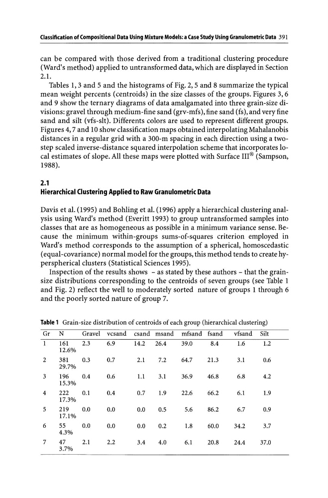
Inspection of the results shows - as stated by these authors - that the grainsize distributions corresponding to the centroids of seven groups (see Table 1
and Fig. 2) reflect the well to moderately sorted nature of groups 1 through 6
and the poorly sorted nature of group 7.
Table 1 Grain-size distribution of centroids of each group (hierarchical clustering)
Gr N
Gravel vcsand csand msand mfsand fsand
vfsand Silt
161
2.3
6.9
14.2
26.4
39.0
8.4
1.6
1.2
12.6%
2
381
0.3
0.7
2.1
7.2
64.7
21.3
3.1
0.6
29.7%
3
196
0.4
0.6
1.1
3.1
36.9
46.8
6.8
4.2
15.3%
4
222
0.1
0.4
0.7
1.9
22.6
66.2
6.1
1.9
17.3%
5
219
0.0
0.0
0.0
0.5
5.6
86.2
6.7
0.9
17.1%
6
55
0.0
0.0
0.0
0.2
1.8
60.0
34.2
3.7
4.3%
7
47
2.1
2.2
3.4
4.0
6.1
20.8
24.4
37.0
3.7%
can be compared with those derived from a traditional clustering procedure
(Ward's method) applied to untransformed data, which are displayed in Section
2.1.
Tables 1, 3 and 5 and the histograms of Fig. 2, 5 and 8 summarize the typical
mean weight percents (centroids) in the size classes of the groups. Figures 3, 6
and 9 show the ternary diagrams of data amalgamated into three grain-size divisions: gravel through medium -fine sand (grv-mfs), fine sand (fs), and very fine
sand and silt (vfs-slt). Differents colors are used to represent different groups.
Figures 4, 7 and 10 show classification maps obtained interpolating Mahalanobis
distances in a regular grid with a 300-m spacing in each direction using a twostep scaled inverse-distance squared interpolation scheme that incorporates local estimates of slope. All these maps were plotted with Surface III® (Sampson,
1988).
2.1
Hierarchical Clustering Applied to Raw Granulometric Data
Davis et al. (1995) and Bohling et al. (1996) apply a hierarchical clustering analysis using Ward's method (Everitt 1993) to group untransformed samples into
classes that are as homogeneous as possible in a minimum variance sense. Because the minimum within-groups sums-of-squares criterion employed in
Ward's method corresponds to the assumption of a spherical, homoscedastic
(equal-covariance) normal model for the groups, this method tends to create hyperspherical clusters (Statistical Sciences 1995).
Inspection of the results shows - as stated by these authors - that the grainsize distributions corresponding to the centroids of seven groups (see Table 1
and Fig. 2) reflect the well to moderately sorted nature of groups 1 through 6
and the poorly sorted nature of group 7.
Table 1 Grain-size distribution of centroids of each group (hierarchical clustering)
Gr N
Gravel vcsand csand msand mfsand fsand
vfsand Silt
161
2.3
6.9
14.2
26.4
39.0
8.4
1.6
1.2
12.6%
2
381
0.3
0.7
2.1
7.2
64.7
21.3
3.1
0.6
29.7%
3
196
0.4
0.6
1.1
3.1
36.9
46.8
6.8
4.2
15.3%
4
222
0.1
0.4
0.7
1.9
22.6
66.2
6.1
1.9
17.3%
5
219
0.0
0.0
0.0
0.5
5.6
86.2
6.7
0.9
17.1%
6
55
0.0
0.0
0.0
0.2
1.8
60.0
34.2
3.7
4.3%
7
47
2.1
2.2
3.4
4.0
6.1
20.8
24.4
37.0
3.7%