

Field and Numerical Studies of Near-Bed Aggregate Dynamics
193
6
Aggregate Disaggregation
Strong gradients of current velocity lead to turbulence and increasing shear
stress. The resulting relative motion between an aggregate and the fluid is largest
close to the seafloor. Thus, it is most likely that aggregates are destroyed in this
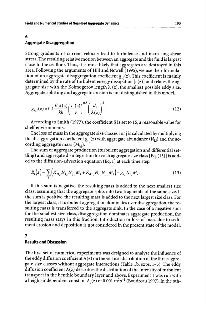
area. Following the arguments of Hill and Nowell (1995), we use their formulation of an aggregate disaggregation coefficient gi,j(Z). This coefficient is mainly
determined by the rate of turbulent energy dissipation [E(Z)] and relates the aggregate size with the Kolmogorov length J.... (z), the smallest possible eddy size.
Aggregate splitting and aggregate erosion is not distinguished in this model.
.. (z) = 0.1 f3 A(Z) (~)O.5(~)2
gz,j
kh
v
A(Z)
(12)
According to Smith (1977), the coefficient ~ is set to 15, a reasonable value for
shelf environments.
The loss of mass in the aggregate size classes i or j is calculated by multiplying
the disaggregation coefficient gi,j(Z) with aggregate abundance (Ni,j) and the according aggregate mass (Mi,j).
The sum of aggregate production (turbulent aggregation and differential settling) and aggregate disintegration for each aggregate size class [Eq. (13)] is added to the diffusion-advection equation (Eq. 1) at each time step.
(13)
If this sum is negative, the resulting mass is added to the next smallest size
class, assuming that the aggregate splits into two fragments of the same size. If
the sum is positive, the resulting mass is added to the next largest size class. For
the largest class, if turbulent aggregation dominates over disaggregation, the resulting mass is transferred to the aggregate sink. In the case of a negative sum
for the smallest size class, disaggregation dominates aggregate production, the
resulting mass stays in this fraction. Introduction or loss of mass due to sediment erosion and deposition is not considered in the present state of the model.
7
Results and Discussion
The first set of numerical experiments was designed to analyse the influence of
the eddy diffusion coefficient A(z) on the vertical distribution of the three aggregate size classes without aggregate interactions (Table 1b, exps. 1-5). The eddy
diffusion coefficient A(z) describes the distribution of the intensity of turbulent
transport in the benthic boundary layer and above. Experiment 1 was run with
a height-independent constant A,(z) of 0.00 1 m 2 S-1 (Boudreau 1997). In the oth-
193
6
Aggregate Disaggregation
Strong gradients of current velocity lead to turbulence and increasing shear
stress. The resulting relative motion between an aggregate and the fluid is largest
close to the seafloor. Thus, it is most likely that aggregates are destroyed in this
area. Following the arguments of Hill and Nowell (1995), we use their formulation of an aggregate disaggregation coefficient gi,j(Z). This coefficient is mainly
determined by the rate of turbulent energy dissipation [E(Z)] and relates the aggregate size with the Kolmogorov length J.... (z), the smallest possible eddy size.
Aggregate splitting and aggregate erosion is not distinguished in this model.
.. (z) = 0.1 f3 A(Z) (~)O.5(~)2
gz,j
kh
v
A(Z)
(12)
According to Smith (1977), the coefficient ~ is set to 15, a reasonable value for
shelf environments.
The loss of mass in the aggregate size classes i or j is calculated by multiplying
the disaggregation coefficient gi,j(Z) with aggregate abundance (Ni,j) and the according aggregate mass (Mi,j).
The sum of aggregate production (turbulent aggregation and differential settling) and aggregate disintegration for each aggregate size class [Eq. (13)] is added to the diffusion-advection equation (Eq. 1) at each time step.
(13)
If this sum is negative, the resulting mass is added to the next smallest size
class, assuming that the aggregate splits into two fragments of the same size. If
the sum is positive, the resulting mass is added to the next largest size class. For
the largest class, if turbulent aggregation dominates over disaggregation, the resulting mass is transferred to the aggregate sink. In the case of a negative sum
for the smallest size class, disaggregation dominates aggregate production, the
resulting mass stays in this fraction. Introduction or loss of mass due to sediment erosion and deposition is not considered in the present state of the model.
7
Results and Discussion
The first set of numerical experiments was designed to analyse the influence of
the eddy diffusion coefficient A(z) on the vertical distribution of the three aggregate size classes without aggregate interactions (Table 1b, exps. 1-5). The eddy
diffusion coefficient A(z) describes the distribution of the intensity of turbulent
transport in the benthic boundary layer and above. Experiment 1 was run with
a height-independent constant A,(z) of 0.00 1 m 2 S-1 (Boudreau 1997). In the oth-