

Lagrangian Modelling Techniques Simulating Wave and Sediment Dynamics ...
5
with a sediment dynamics model provides for calculation of sediment transport
in wave and current environments.
WGEN3DD acts by subdividing the fetch along the wind direction into short
lengths of order 10-100 m. In each segment, empirical formulae for wave generation are applied to find the theoretical heights and periods. The model incorporates linear wave shoaling and then truncates the height if it exceeds the
breaking depth limitation. Steepness limited truncation of the spectrum can be
simulated (Black 1997) but was not applied in this study. The effect of shoaling,
breaking and friction is accumulated in each segment to produce the hindcast
wave heights along the fetch. The frictional dissipation is calculated by adopting
the formulae of Bretschneider and Reid (1954). To obtain bottom orbital currents from sea surface wave height, the theoretical JONSWAP spectrum is decomposed into frequency intervals ilf and the linear theory wave transform is
applied to each frequency band. A regular time series of bed orbital currents is
reconstituted at 2 Hz by linear summation of the transformed spectral components (assuming a random phase for each component). For sediment transport
calculations, the third velocity moment defined by Black and Rosenberg (1991)
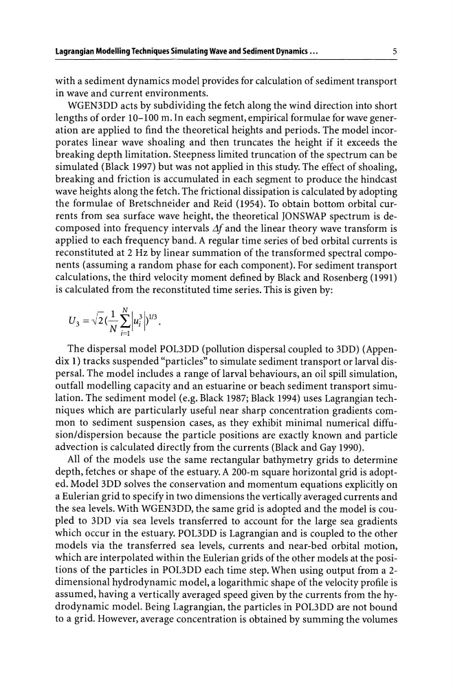
is calculated from the reconstituted time series. This is given by:
N
U3 = fi(~ ~HI)1/3.
The dispersal model POL3DD (pollution dispersal coupled to 3DD) (Appendix 1) tracks suspended "particles" to simulate sediment transport or larval dispersal. The model includes a range of larval behaviours, an oil spill simulation,
outfall modelling capacity and an estuarine or beach sediment transport simulation. The sediment model (e.g. Black 1987; Black 1994) uses Lagrangian techniques which are particularly useful near sharp concentration gradients common to sediment suspension cases, as they exhibit minimal numerical diffusion/dispersion because the particle positions are exactly known and particle
advection is calculated directly from the currents (Black and Gay 1990).
All of the models use the same rectangular bathymetry grids to determine
depth, fetches or shape of the estuary. A 200-m square horizontal grid is adopted. Model 3DD solves the conservation and momentum equations explicitly on
a Eulerian grid to specify in two dimensions the vertically averaged currents and
the sea levels. With WGEN3DD, the same grid is adopted and the model is coupled to 3DD via sea levels transferred to account for the large sea gradients
which occur in the estuary. POL3DD is Lagrangian and is coupled to the other
models via the transferred sea levels, currents and near-bed orbital motion,
which are interpolated within the Eulerian grids of the other models at the positions of the particles in POL3DD each time step. When using output from a 2dimensional hydrodynamic model, a logarithmic shape of the velocity profile is
assumed, having a vertically averaged speed given by the currents from the hydrodynamic model. Being Lagrangian, the particles in POL3DD are not bound
to a grid. However, average concentration is obtained by summing the volumes
5
with a sediment dynamics model provides for calculation of sediment transport
in wave and current environments.
WGEN3DD acts by subdividing the fetch along the wind direction into short
lengths of order 10-100 m. In each segment, empirical formulae for wave generation are applied to find the theoretical heights and periods. The model incorporates linear wave shoaling and then truncates the height if it exceeds the
breaking depth limitation. Steepness limited truncation of the spectrum can be
simulated (Black 1997) but was not applied in this study. The effect of shoaling,
breaking and friction is accumulated in each segment to produce the hindcast
wave heights along the fetch. The frictional dissipation is calculated by adopting
the formulae of Bretschneider and Reid (1954). To obtain bottom orbital currents from sea surface wave height, the theoretical JONSWAP spectrum is decomposed into frequency intervals ilf and the linear theory wave transform is
applied to each frequency band. A regular time series of bed orbital currents is
reconstituted at 2 Hz by linear summation of the transformed spectral components (assuming a random phase for each component). For sediment transport
calculations, the third velocity moment defined by Black and Rosenberg (1991)
is calculated from the reconstituted time series. This is given by:
N
U3 = fi(~ ~HI)1/3.
The dispersal model POL3DD (pollution dispersal coupled to 3DD) (Appendix 1) tracks suspended "particles" to simulate sediment transport or larval dispersal. The model includes a range of larval behaviours, an oil spill simulation,
outfall modelling capacity and an estuarine or beach sediment transport simulation. The sediment model (e.g. Black 1987; Black 1994) uses Lagrangian techniques which are particularly useful near sharp concentration gradients common to sediment suspension cases, as they exhibit minimal numerical diffusion/dispersion because the particle positions are exactly known and particle
advection is calculated directly from the currents (Black and Gay 1990).
All of the models use the same rectangular bathymetry grids to determine
depth, fetches or shape of the estuary. A 200-m square horizontal grid is adopted. Model 3DD solves the conservation and momentum equations explicitly on
a Eulerian grid to specify in two dimensions the vertically averaged currents and
the sea levels. With WGEN3DD, the same grid is adopted and the model is coupled to 3DD via sea levels transferred to account for the large sea gradients
which occur in the estuary. POL3DD is Lagrangian and is coupled to the other
models via the transferred sea levels, currents and near-bed orbital motion,
which are interpolated within the Eulerian grids of the other models at the positions of the particles in POL3DD each time step. When using output from a 2dimensional hydrodynamic model, a logarithmic shape of the velocity profile is
assumed, having a vertically averaged speed given by the currents from the hydrodynamic model. Being Lagrangian, the particles in POL3DD are not bound
to a grid. However, average concentration is obtained by summing the volumes