

11 The RADARSAT Geophysical Processor System
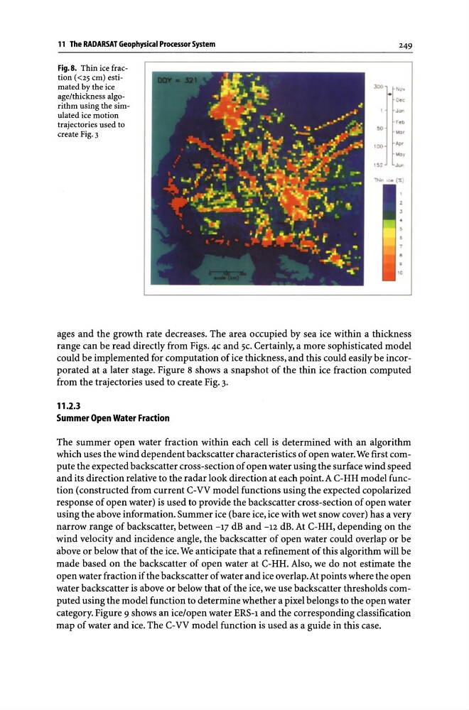
Fig.8. Thin ice fraction «25 em) estimated by the ice
age/thickness algorithm using the simulated ice motion
trajectories used to
create Fig. 3
JOO
:10
'00
.51
249
~ ...
C
reo
... '
.".
"01
J ...
ages and the growth rate decreases. The area occupied by sea ice within a thickness
range can be read directly from Figs. 4C and 5C. Certainly, a more sophisticated model
could be implemented for computation of ice thickness, and this could easily be incorporated at a later stage. Figure 8 shows a snapshot of the thin ice fraction computed
from the trajectories used to create Fig. 3.
11.2.3
Summer Open Water Fraction
The summer open water fraction within each cell is determined with an algorithm
which uses the wind dependent backscatter characteristics of open water. We first compute the expected backscatter cross-section of open water using the surface wind speed
and its direction relative to the radar look direction at each point. A C-HH model function (constructed from current C-VV model functions using the expected copolarized
response of open water) is used to provide the backscatter cross-section of open water
using the above information. Summer ice (bare ice, ice with wet snow cover) has a very
narrow range of backscatter, between -17 dB and -l2 dB. At C-HH, depending on the
wind velocity and incidence angle, the backscatter of open water could overlap or be
above or below that of the ice. We anticipate that a refinement of this algorithm will be
made based on the backscatter of open water at C-HH. Also, we do not estimate the
open water fraction if the backscatter of water and ice overlap. At points where the open
water backscatter is above or below that of the ice, we use backscatter thresholds computed using the model function to determine whether a pixel belongs to the open water
category. Figure 9 shows an ice/open water ERS-1 and the corresponding classification
map of water and ice. The C-VV model function is used as a guide in this case.
Fig.8. Thin ice fraction «25 em) estimated by the ice
age/thickness algorithm using the simulated ice motion
trajectories used to
create Fig. 3
JOO
:10
'00
.51
249
~ ...
C
reo
... '
.".
"01
J ...
ages and the growth rate decreases. The area occupied by sea ice within a thickness
range can be read directly from Figs. 4C and 5C. Certainly, a more sophisticated model
could be implemented for computation of ice thickness, and this could easily be incorporated at a later stage. Figure 8 shows a snapshot of the thin ice fraction computed
from the trajectories used to create Fig. 3.
11.2.3
Summer Open Water Fraction
The summer open water fraction within each cell is determined with an algorithm
which uses the wind dependent backscatter characteristics of open water. We first compute the expected backscatter cross-section of open water using the surface wind speed
and its direction relative to the radar look direction at each point. A C-HH model function (constructed from current C-VV model functions using the expected copolarized
response of open water) is used to provide the backscatter cross-section of open water
using the above information. Summer ice (bare ice, ice with wet snow cover) has a very
narrow range of backscatter, between -17 dB and -l2 dB. At C-HH, depending on the
wind velocity and incidence angle, the backscatter of open water could overlap or be
above or below that of the ice. We anticipate that a refinement of this algorithm will be
made based on the backscatter of open water at C-HH. Also, we do not estimate the
open water fraction if the backscatter of water and ice overlap. At points where the open
water backscatter is above or below that of the ice, we use backscatter thresholds computed using the model function to determine whether a pixel belongs to the open water
category. Figure 9 shows an ice/open water ERS-1 and the corresponding classification
map of water and ice. The C-VV model function is used as a guide in this case.