

216
C. BERTOIA, J. FALKINGHAM, F. FETTERER
pretation of image features, absolute image calibration is not required. In fact, quantitative ice analysis from SAR is not be considered viable until the advent of the Intera
STAR-1 radar in Canada. This system, the first that could be calibrated, began service
as a sea ice imaging radar in 1986, but operational data communications procedures
made absolute calibration, or even relative calibration, of this system infrequent (Livingstone 1994).
10.5.1
Backscatter for Ice Classification
Although ice thickness is not directly derivable from single frequency/single polarization SAR, techniques have been developed that make classification of ice into stages of
development possible. The stages of ice development have been defined into standard
categories by the World Meteorological Organization based on ice tlIickness and ice age
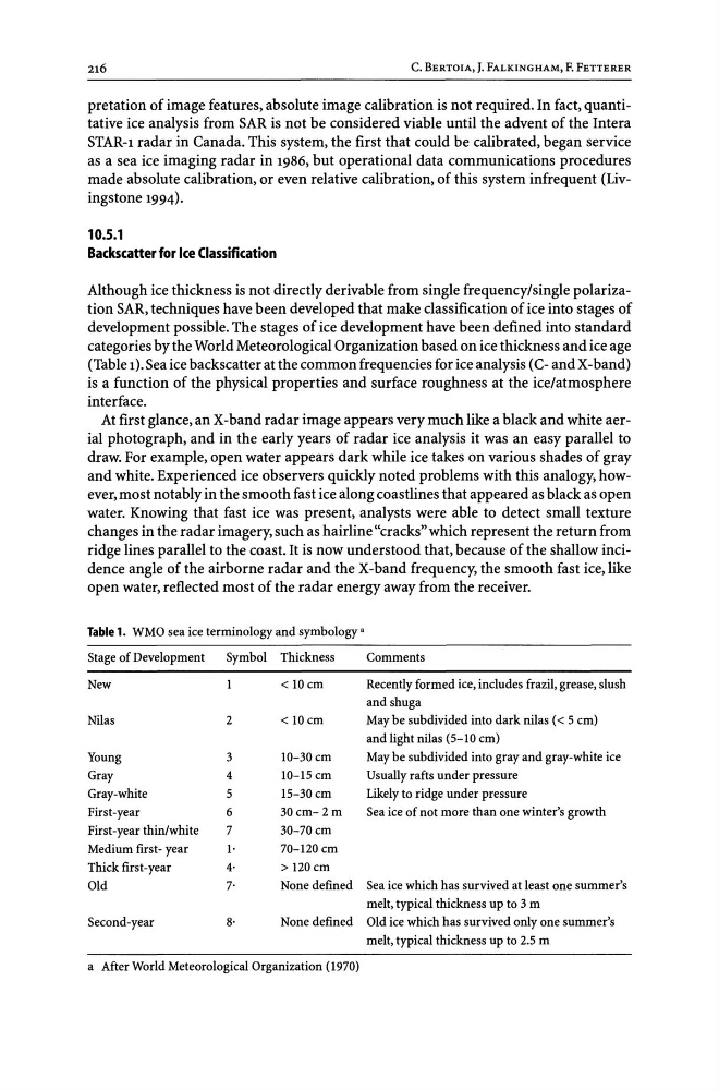
(Table 1). Sea ice backscatter at the common frequencies for ice analysis (C- and X-band)
is a function of the physical properties and surface roughness at the ice/atmosphere
interface.
At first glance, an X-band radar image appears very much like a black and white aerial photograph, and in the early years of radar ice analysis it was an easy parallel to
draw. For example, open water appears dark while ice takes on various shades of gray
and white. Experienced ice observers quickly noted problems with this analogy, however, most notably in the smooth fast ice along coastlines that appeared as black as open
water. Knowing that fast ice was present, analysts were able to detect small texture
changes in the radar imagery, such as hairline "cracks" which represent the return from
ridge lines parallel to the coast. It is now understood that, because of the shallow incidence angle of the airborne radar and the X-band frequency, the smooth fast ice, like
open water, reflected most of the radar energy away from the receiver.
Table 1. WMO sea ice terminology and symbology a
Stage of Development
Symbol Thickness
New
< lOcm
Nilas
2
< 10cm
Young
3
10-30 cm
Gray
4
10-15 cm
Gray-white
5
15-30 cm
First-year
6
30cm-2m
First-year thin/white
7
30-70 cm
Medium first-year
1·
70-120 cm
Thick first-year
4·
> 120 cm
Old
7'
None defined
Second-year
8·
None defined
a After World Meteorological Organization (1970)
Comments
Recently formed ice, includes frazil, grease, slush
andshuga
May be subdivided into dark nilas « 5 cm)
and light nilas (5-10 cm)
May be subdivided into gray and gray-white ice
Usually rafts under pressure
Likely to ridge under pressure
Sea ice of not more than one winter's growth
Sea ice which has survived at least one summer's
melt, typical thickness up to 3 m
Old ice which has survived only one summer's
melt, typical thickness up to 2.5 m
C. BERTOIA, J. FALKINGHAM, F. FETTERER
pretation of image features, absolute image calibration is not required. In fact, quantitative ice analysis from SAR is not be considered viable until the advent of the Intera
STAR-1 radar in Canada. This system, the first that could be calibrated, began service
as a sea ice imaging radar in 1986, but operational data communications procedures
made absolute calibration, or even relative calibration, of this system infrequent (Livingstone 1994).
10.5.1
Backscatter for Ice Classification
Although ice thickness is not directly derivable from single frequency/single polarization SAR, techniques have been developed that make classification of ice into stages of
development possible. The stages of ice development have been defined into standard
categories by the World Meteorological Organization based on ice tlIickness and ice age
(Table 1). Sea ice backscatter at the common frequencies for ice analysis (C- and X-band)
is a function of the physical properties and surface roughness at the ice/atmosphere
interface.
At first glance, an X-band radar image appears very much like a black and white aerial photograph, and in the early years of radar ice analysis it was an easy parallel to
draw. For example, open water appears dark while ice takes on various shades of gray
and white. Experienced ice observers quickly noted problems with this analogy, however, most notably in the smooth fast ice along coastlines that appeared as black as open
water. Knowing that fast ice was present, analysts were able to detect small texture
changes in the radar imagery, such as hairline "cracks" which represent the return from
ridge lines parallel to the coast. It is now understood that, because of the shallow incidence angle of the airborne radar and the X-band frequency, the smooth fast ice, like
open water, reflected most of the radar energy away from the receiver.
Table 1. WMO sea ice terminology and symbology a
Stage of Development
Symbol Thickness
New
< lOcm
Nilas
2
< 10cm
Young
3
10-30 cm
Gray
4
10-15 cm
Gray-white
5
15-30 cm
First-year
6
30cm-2m
First-year thin/white
7
30-70 cm
Medium first-year
1·
70-120 cm
Thick first-year
4·
> 120 cm
Old
7'
None defined
Second-year
8·
None defined
a After World Meteorological Organization (1970)
Comments
Recently formed ice, includes frazil, grease, slush
andshuga
May be subdivided into dark nilas « 5 cm)
and light nilas (5-10 cm)
May be subdivided into gray and gray-white ice
Usually rafts under pressure
Likely to ridge under pressure
Sea ice of not more than one winter's growth
Sea ice which has survived at least one summer's
melt, typical thickness up to 3 m
Old ice which has survived only one summer's
melt, typical thickness up to 2.5 m