

7 Mapping the Progression of Melt Onset and Freeze-Up
137
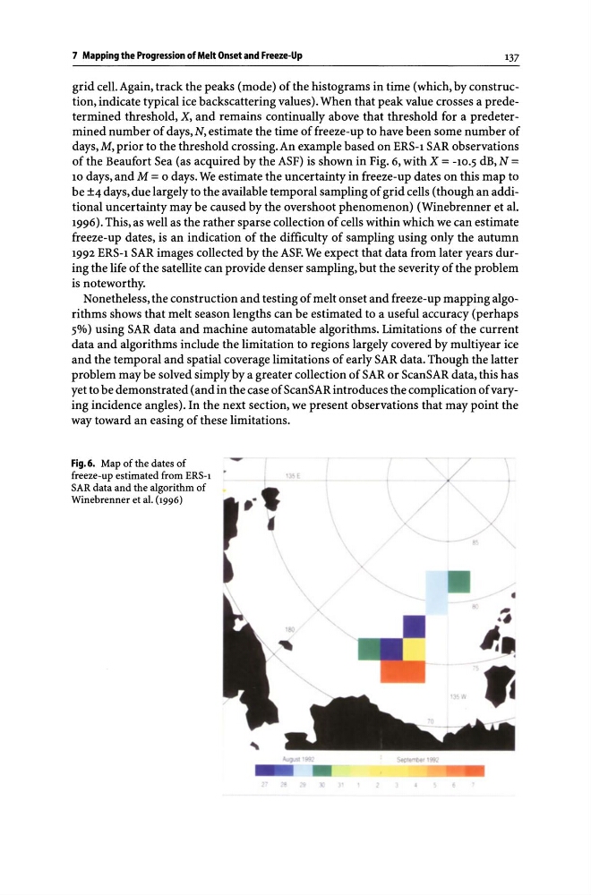
grid celL Again, track the peaks (mode) of the histograms in time (which, byconstruction, indicate typical ice backscattering values) _ When that peak value crosses a predetermined threshold, X, and remains continually above that threshold for a predetermined number of days, N, estimate the time of freeze-up to have been some number of
days, M, prior to the threshold crossing_ An example based on ERS-l SAR observations
of the Beaufort Sea (as acquired by the ASF) is shown in Fig. 6, with X = -10.5 dB, N =
10 days, and M = 0 days. We estimate the uncertainty in freeze-up dates on this map to
be ±4 days, due largely to the available temporal sampling of grid cells (though an additional uncertainty may be caused by the overshoot phenomenon) (Winebrenner et al.
1996). This, as well as the rather sparse collection of cells within which we can estimate
freeze-up dates, is an indication of the difficulty of sampling using only the autumn
1992 ERS-l SAR images collected by the ASF. We expect that data from later years during the life of the satellite can provide denser sampling, but the severity of the problem
is noteworthy.
Nonetheless, the construction and testing of melt onset and freeze-up mapping algorithms shows that melt season lengths can be estimated to a useful accuracy (perhaps
5%) using SAR data and machine automatable algorithms. Limitations of the current
data and algorithms include the limitation to regions largely covered by multiyear ice
and the temporal and spatial coverage limitations of early SAR data. Though the latter
problem may be solved simply by a greater collection of SAR or ScanSAR data, this has
yet to be demonstrated (and in the case of ScanSAR introduces the complication of varying incidence angles). In the next section, we present observations that may point the
way toward an easing of these limitations.
Fig.6. Map of the dates of
freeze-up estimated from ERS-l •
SAR data and the algorithm of
Winebrenner et al. (1996)
-
/
137
grid celL Again, track the peaks (mode) of the histograms in time (which, byconstruction, indicate typical ice backscattering values) _ When that peak value crosses a predetermined threshold, X, and remains continually above that threshold for a predetermined number of days, N, estimate the time of freeze-up to have been some number of
days, M, prior to the threshold crossing_ An example based on ERS-l SAR observations
of the Beaufort Sea (as acquired by the ASF) is shown in Fig. 6, with X = -10.5 dB, N =
10 days, and M = 0 days. We estimate the uncertainty in freeze-up dates on this map to
be ±4 days, due largely to the available temporal sampling of grid cells (though an additional uncertainty may be caused by the overshoot phenomenon) (Winebrenner et al.
1996). This, as well as the rather sparse collection of cells within which we can estimate
freeze-up dates, is an indication of the difficulty of sampling using only the autumn
1992 ERS-l SAR images collected by the ASF. We expect that data from later years during the life of the satellite can provide denser sampling, but the severity of the problem
is noteworthy.
Nonetheless, the construction and testing of melt onset and freeze-up mapping algorithms shows that melt season lengths can be estimated to a useful accuracy (perhaps
5%) using SAR data and machine automatable algorithms. Limitations of the current
data and algorithms include the limitation to regions largely covered by multiyear ice
and the temporal and spatial coverage limitations of early SAR data. Though the latter
problem may be solved simply by a greater collection of SAR or ScanSAR data, this has
yet to be demonstrated (and in the case of ScanSAR introduces the complication of varying incidence angles). In the next section, we present observations that may point the
way toward an easing of these limitations.
Fig.6. Map of the dates of
freeze-up estimated from ERS-l •
SAR data and the algorithm of
Winebrenner et al. (1996)
-
/