

124
A. K. LIU AND C. Y. PENG
days 21 and 24,1992, near St. Lawrence Island. Then, each closed contour is indexed and
framed in a rectangular window with its four sides just tangent to the four extreme
locations of the closed contour respectively. For each window, a binary image is generated with those pixels within the boundary set to one and those outside the boundary
but within the rectangle set to zero. We also select a closed contour at the starting date
as the template of the ice floe. In this study, we selected a prominent contour, number
16 in Fig. lOa, as the initial ice floe.
We then perform template matching on the binary image of the template with each
instance of binary image 3 days later (day 24, Fig. lOb). The two binary images are first
superimposed at their respective center of mass. For template matching, a metric which
measures the degree of mismatch between the template and an unknown pattern is
defined as follows (Schalkoff 1992):
where f denotes the template pattern, g is the unknown target pattern, and R is the range
of the template pattern,f, namely, the window enclosing the closed contour for the template.A small value of m indicates two patterns are similar, while a large value of m indicates they are different. Because the shapes of the ice floes are in the form of binary images,
f and g are both in binary digits. Thus the metric in Eq. (3) can be further simplified by:
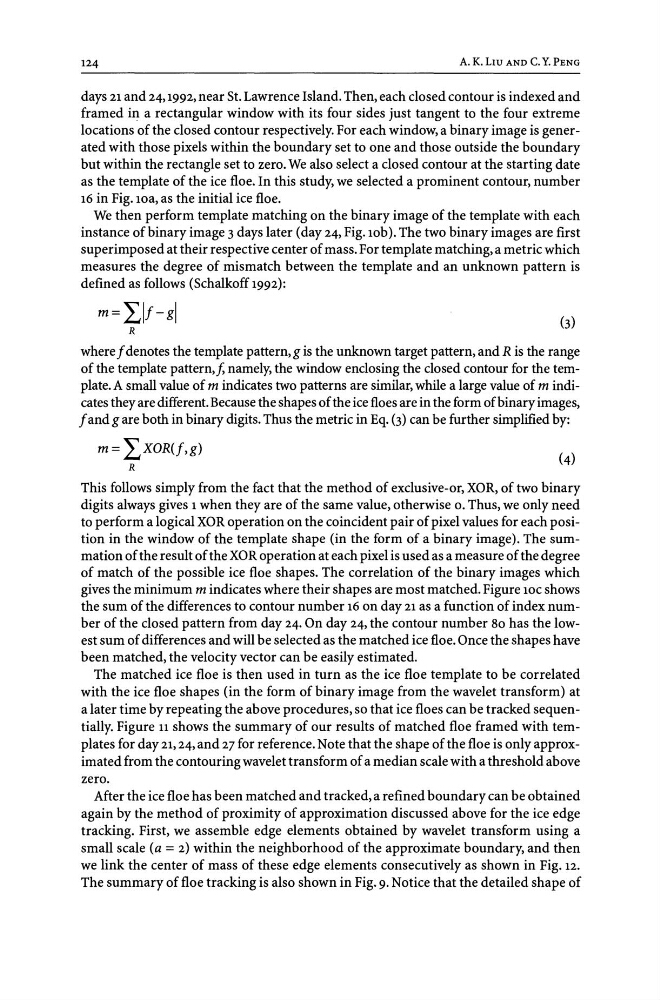
m = LXOR(j,g)
R
This follows simply from the fact that the method of exclusive-or, XOR, of two binary
digits always gives 1 when they are of the same value, otherwise o. Thus, we only need
to perform a logical XOR operation on the coincident pair of pixel values for each position in the window of the template shape (in the form of a binary image). The summation of the result of the XOR operation at each pixel is used as a measure of the degree
of match of the possible ice floe shapes. The correlation of the binary images which
gives the minimum m indicates where their shapes are most matched. Figure 10C shows
the sum of the differences to contour number 16 on day 21 as a function of index number of the closed pattern from day 24. On day 24, the contour number 80 has the lowest sum of differences and will be selected as the matched ice floe. Once the shapes have
been matched, the velocity vector can be easily estimated.
The matched ice floe is then used in turn as the ice floe template to be correlated
with the ice floe shapes (in the form of binary image from the wavelet transform) at
a later time by repeating the above procedures, so that ice floes can be tracked sequentially. Figure 11 shows the summary of our results of matched floe framed with templates for day 21, 24, and 27 for reference. Note that the shape of the floe is onlyapproximated from the contouring wavelet transform of a median scale with a threshold above
zero.
After the ice floe has been matched and tracked, a refined boundary can be obtained
again by the method of proximity of approximation discussed above for the ice edge
tracking. First, we assemble edge elements obtained by wavelet transform using a
small scale (a = 2) within the neighborhood of the approximate boundary, and then
we link the center of mass of these edge elements consecutively as shown in Fig. 12.
The summary of floe tracking is also shown in Fig. 9. Notice that the detailed shape of
A. K. LIU AND C. Y. PENG
days 21 and 24,1992, near St. Lawrence Island. Then, each closed contour is indexed and
framed in a rectangular window with its four sides just tangent to the four extreme
locations of the closed contour respectively. For each window, a binary image is generated with those pixels within the boundary set to one and those outside the boundary
but within the rectangle set to zero. We also select a closed contour at the starting date
as the template of the ice floe. In this study, we selected a prominent contour, number
16 in Fig. lOa, as the initial ice floe.
We then perform template matching on the binary image of the template with each
instance of binary image 3 days later (day 24, Fig. lOb). The two binary images are first
superimposed at their respective center of mass. For template matching, a metric which
measures the degree of mismatch between the template and an unknown pattern is
defined as follows (Schalkoff 1992):
where f denotes the template pattern, g is the unknown target pattern, and R is the range
of the template pattern,f, namely, the window enclosing the closed contour for the template.A small value of m indicates two patterns are similar, while a large value of m indicates they are different. Because the shapes of the ice floes are in the form of binary images,
f and g are both in binary digits. Thus the metric in Eq. (3) can be further simplified by:
m = LXOR(j,g)
R
This follows simply from the fact that the method of exclusive-or, XOR, of two binary
digits always gives 1 when they are of the same value, otherwise o. Thus, we only need
to perform a logical XOR operation on the coincident pair of pixel values for each position in the window of the template shape (in the form of a binary image). The summation of the result of the XOR operation at each pixel is used as a measure of the degree
of match of the possible ice floe shapes. The correlation of the binary images which
gives the minimum m indicates where their shapes are most matched. Figure 10C shows
the sum of the differences to contour number 16 on day 21 as a function of index number of the closed pattern from day 24. On day 24, the contour number 80 has the lowest sum of differences and will be selected as the matched ice floe. Once the shapes have
been matched, the velocity vector can be easily estimated.
The matched ice floe is then used in turn as the ice floe template to be correlated
with the ice floe shapes (in the form of binary image from the wavelet transform) at
a later time by repeating the above procedures, so that ice floes can be tracked sequentially. Figure 11 shows the summary of our results of matched floe framed with templates for day 21, 24, and 27 for reference. Note that the shape of the floe is onlyapproximated from the contouring wavelet transform of a median scale with a threshold above
zero.
After the ice floe has been matched and tracked, a refined boundary can be obtained
again by the method of proximity of approximation discussed above for the ice edge
tracking. First, we assemble edge elements obtained by wavelet transform using a
small scale (a = 2) within the neighborhood of the approximate boundary, and then
we link the center of mass of these edge elements consecutively as shown in Fig. 12.
The summary of floe tracking is also shown in Fig. 9. Notice that the detailed shape of