

4.1 Non-Linear Energy Transfer in Wind Wave Spectrum
87
The most optimal integration algorithm, making the present method different from the others (Hasselmann & Hasselmann, 1981; Masuda, 1981; Komatsu&Masuda, 1996; Polnikov, 1989; Resio&Perrie, 1991) can be based on
utilization of the Jacobi weight functions (Krylov & Shulgina, 1966).
The integration is carried out within the range 0.5aa(1- ca/2) ~ a2 ~
0.5aa (1- .../ca -1) in case ca > 1 (where ca = 2ka/a~). There are two
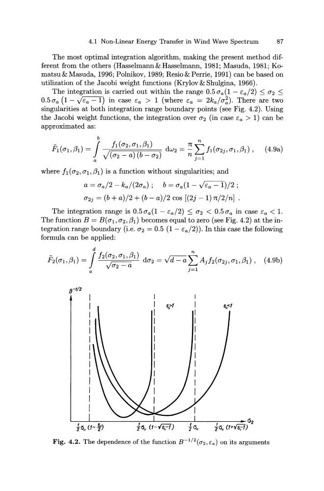
singularities at both integration range boundary points (see Fig. 4.2). Using
the Jacobi weight functions, the integration over a2 (in case ca > 1) can be
approximated as:
n
--r:F====~~===~ dw2 = ~ L h ( a2j, at, ,BI) ,
n j=l
where h ( a2, at, ,61 ) is a function without singularities; and
a= aa/2- ka/(2aa); b = aa(1- Vca -1)/2;
a2 1 = (b + a)/2 + (b- a)/2 cos [(2j- 1) 7t/2/n] .
(4.9a)
The integration range is 0.5aa(1- ca/2) ~ a2 < 0.5aa in case ca < 1.
The function B = B(at, a2, ,BI) becomes equal to zero (see Fig. 4.2) at the integration range boundary (i.e. a2 = 0.5 (1- ca/2)). In this case the following
formula can be applied:
(4.9b)
Fig. 4.2. The dependence of the function s- 1 / 2 (u2 , ca) on its arguments
87
The most optimal integration algorithm, making the present method different from the others (Hasselmann & Hasselmann, 1981; Masuda, 1981; Komatsu&Masuda, 1996; Polnikov, 1989; Resio&Perrie, 1991) can be based on
utilization of the Jacobi weight functions (Krylov & Shulgina, 1966).
The integration is carried out within the range 0.5aa(1- ca/2) ~ a2 ~
0.5aa (1- .../ca -1) in case ca > 1 (where ca = 2ka/a~). There are two
singularities at both integration range boundary points (see Fig. 4.2). Using
the Jacobi weight functions, the integration over a2 (in case ca > 1) can be
approximated as:
n
--r:F====~~===~ dw2 = ~ L h ( a2j, at, ,BI) ,
n j=l
where h ( a2, at, ,61 ) is a function without singularities; and
a= aa/2- ka/(2aa); b = aa(1- Vca -1)/2;
a2 1 = (b + a)/2 + (b- a)/2 cos [(2j- 1) 7t/2/n] .
(4.9a)
The integration range is 0.5aa(1- ca/2) ~ a2 < 0.5aa in case ca < 1.
The function B = B(at, a2, ,BI) becomes equal to zero (see Fig. 4.2) at the integration range boundary (i.e. a2 = 0.5 (1- ca/2)). In this case the following
formula can be applied:
(4.9b)
Fig. 4.2. The dependence of the function s- 1 / 2 (u2 , ca) on its arguments