

3.7 Numerical Integration of the Source Function
73
RMS
1.00000
010000
0.01000
--+- -1
0.00100
- - - -2
-8- -3
0.00
20000.00
40000.00
60000.00
80000.00
100000.00
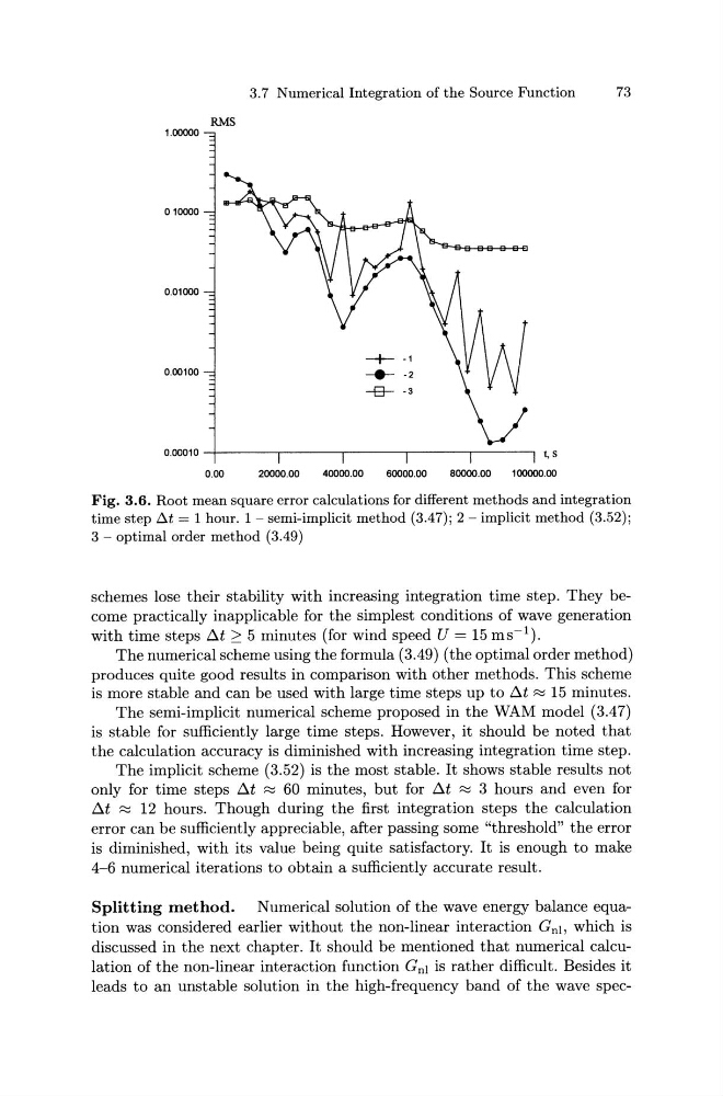
Fig. 3.6. Root mean square error calculations for different methods and integration
time step tlt = 1 hour. 1 ~semi-implicit method (3.47); 2 ~implicit method (3.52);
3 ~optimal order method (3.49)
schemes lose their stability with increasing integration time step. They become practically inapplicable for the simplest conditions of wave generation
with time steps .6.t 2' : 5 minutes (for wind speed U = 15 ms~ 1 ).
The numerical scheme using the formula (3.49) (the optimal order method)
produces quite good results in comparison with other methods. This scheme
is more stable and can be used with large time steps up to .6.t ~ 15 minutes.
The semi-implicit numerical scheme proposed in the WAM model (3.47)
is stable for sufficiently large time steps. However, it should be noted that
the calculation accuracy is diminished with increasing integration time step.
The implicit scheme (3.52) is the most stable. It shows stable results not
only for time steps .6.t ~ 60 minutes, but for .6.t ~ 3 hours and even for
.6.t ~ 12 hours. Though during the first integration steps the calculation
error can be sufficiently appreciable, after passing some "threshold" the error
is diminished, with its value being quite satisfactory. It is enough to make
4-6 numerical iterations to obtain a sufficiently accurate result.
Splitting method. Numerical solution of the wave energy balance equation was considered earlier without the non-linear interaction Gnh which is
discussed in the next chapter. It should be mentioned that numerical calculation of the non-linear interaction function Gnl is rather difficult. Besides it
leads to an unstable solution in the high-frequency band of the wave spec-
73
RMS
1.00000
010000
0.01000
--+- -1
0.00100
- - - -2
-8- -3
0.00
20000.00
40000.00
60000.00
80000.00
100000.00
Fig. 3.6. Root mean square error calculations for different methods and integration
time step tlt = 1 hour. 1 ~semi-implicit method (3.47); 2 ~implicit method (3.52);
3 ~optimal order method (3.49)
schemes lose their stability with increasing integration time step. They become practically inapplicable for the simplest conditions of wave generation
with time steps .6.t 2' : 5 minutes (for wind speed U = 15 ms~ 1 ).
The numerical scheme using the formula (3.49) (the optimal order method)
produces quite good results in comparison with other methods. This scheme
is more stable and can be used with large time steps up to .6.t ~ 15 minutes.
The semi-implicit numerical scheme proposed in the WAM model (3.47)
is stable for sufficiently large time steps. However, it should be noted that
the calculation accuracy is diminished with increasing integration time step.
The implicit scheme (3.52) is the most stable. It shows stable results not
only for time steps .6.t ~ 60 minutes, but for .6.t ~ 3 hours and even for
.6.t ~ 12 hours. Though during the first integration steps the calculation
error can be sufficiently appreciable, after passing some "threshold" the error
is diminished, with its value being quite satisfactory. It is enough to make
4-6 numerical iterations to obtain a sufficiently accurate result.
Splitting method. Numerical solution of the wave energy balance equation was considered earlier without the non-linear interaction Gnh which is
discussed in the next chapter. It should be mentioned that numerical calculation of the non-linear interaction function Gnl is rather difficult. Besides it
leads to an unstable solution in the high-frequency band of the wave spec-