

s
0.015
0.010
0.005
0.000
0.00
3.7 Numerical Integration of the Source Function
71
1.00
2.00
-e-- 1
-tr- 2
~3
--+- 4
-a- 5
.....-s
3.00
w, rad s- 1
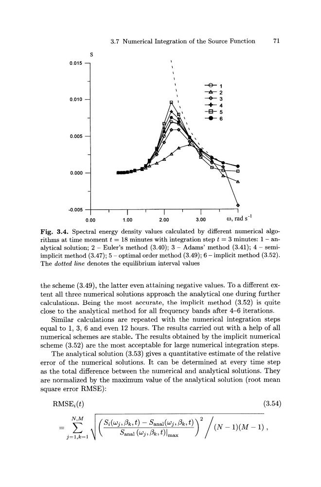
Fig. 3.4. Spectral energy density values calculated by different numerical algorithms at time moment t = 18 minutes with integration step t = 3 minutes: 1 - analytical solution; 2 -Euler's method (3.40); 3- Adams' method (3.41); 4- semiimplicit method (3.47); 5- optimal order method (3.49); 6- implicit method (3.52).
The dotted line denotes the equilibrium interval values
the scheme (3.49), the latter even attaining negative values. To a different extent all three numerical solutions approach the analytical one during further
calculations. Being the most accurate, the implicit method (3.52) is quite
close to the analytical method for all frequency bands after 4-6 iterations.
Similar calculations are repeated with the numerical integration steps
equal to 1, 3, 6 and even 12 hours. The results carried out with a help of all
numerical schemes are stable. The results obtained by the implicit numerical
scheme (3.52) are the most acceptable for large numerical integration steps.
The analytical solution (3.53) gives a quantitative estimate of the relative
error of the numerical solutions. It can be determined at every time step
as the total difference between the numerical and analytical solutions. They
are normalized by the maximum value of the analytical solution (root mean
square error RMSE):
N,M
I:
j=l,k=l
(3.54)
( Si(wj,f3k, t)- Sanal(wj,f3k, t))
2
/(N _ 1 )(M -1),
Banal (wj' f3k, t) I max
0.015
0.010
0.005
0.000
0.00
3.7 Numerical Integration of the Source Function
71
1.00
2.00
-e-- 1
-tr- 2
~3
--+- 4
-a- 5
.....-s
3.00
w, rad s- 1
Fig. 3.4. Spectral energy density values calculated by different numerical algorithms at time moment t = 18 minutes with integration step t = 3 minutes: 1 - analytical solution; 2 -Euler's method (3.40); 3- Adams' method (3.41); 4- semiimplicit method (3.47); 5- optimal order method (3.49); 6- implicit method (3.52).
The dotted line denotes the equilibrium interval values
the scheme (3.49), the latter even attaining negative values. To a different extent all three numerical solutions approach the analytical one during further
calculations. Being the most accurate, the implicit method (3.52) is quite
close to the analytical method for all frequency bands after 4-6 iterations.
Similar calculations are repeated with the numerical integration steps
equal to 1, 3, 6 and even 12 hours. The results carried out with a help of all
numerical schemes are stable. The results obtained by the implicit numerical
scheme (3.52) are the most acceptable for large numerical integration steps.
The analytical solution (3.53) gives a quantitative estimate of the relative
error of the numerical solutions. It can be determined at every time step
as the total difference between the numerical and analytical solutions. They
are normalized by the maximum value of the analytical solution (root mean
square error RMSE):
N,M
I:
j=l,k=l
(3.54)
( Si(wj,f3k, t)- Sanal(wj,f3k, t))
2
/(N _ 1 )(M -1),
Banal (wj' f3k, t) I max