

3.5 Interpolation-Ray (INTERPOL) Method
59
L
L
~ ~ sn+l(wk, ,61)~,6 = 2 ; ~ {vSn(wk, ,61-1) + (1- 2v)Sn(wk, ,61)
1=1
1=1
(3.25)
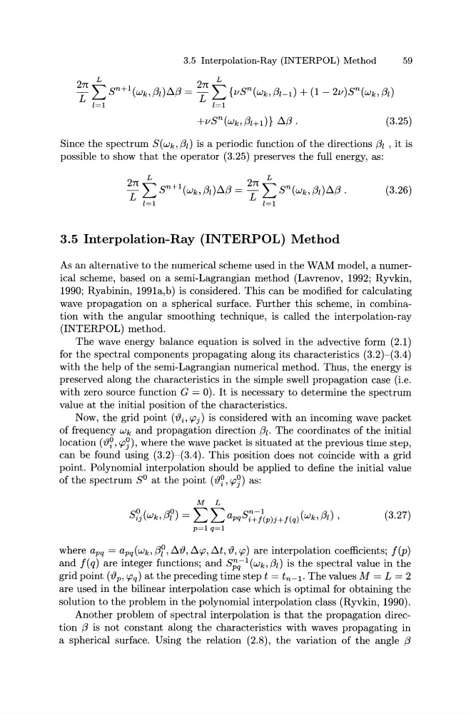
Since the spectrum S(wk, ,61) is a periodic function of the directions ,61 , it is
possible to show that the operator (3.25) preserves the full energy, as:
L
L
2 ; ~ sn+ 1 (wk,,61)~,6 = ~ ~ sn(wk,,6z)~,6.
1=1
1=1
(3.26)
3.5 Interpolation-Ray (INTERPOL) Method
As an alternative to the numerical scheme used in the WAM model, a numerical scheme, based on a semi-Lagrangian method (Lavrenov, 1992; Ryvkin,
1990; Ryabinin, 1991a,b) is considered. This can be modified for calculating
wave propagation on a spherical surface. Further this scheme, in combination with the angular smoothing technique, is called the interpolation-ray
(INTERPOL) method.
The wave energy balance equation is solved in the advective form (2.1)
for the spectral components propagating along its characteristics (3.2)-(3.4)
with the help of the semi-Lagrangian numerical method. Thus, the energy is
preserved along the characteristics in the simple swell propagation case (i.e.
with zero source function G = 0). It is necessary to determine the spectrum
value at the initial position of the characteristics.
Now, the grid point ( {) i, ip j) is considered with an incoming wave packet
of frequency Wk and propagation direction ,61. The coordinates of the initial
location ( 1J?, IPj), where the wave packet is situated at the previous time step,
can be found using (3.2)-(3.4). This position does not coincide with a grid
point. Polynomial interpolation should be applied to define the initial value
of the spectrum S 0 at the point ( 1J?, IPJ) as:
M
L
sfj(wk,,LJ?) = ~~apqs~+-Ap)J+t(q)(wk,,61),
(3.27)
p=1q=1
where apq = apq(wk, ,6p, ~{), ~ip, ~t, 1J, IP) are interpolation coefficients; f(p)
and f(q) are integer functions; and s;q- 1 (wk?,6z) is the spectral value in the
grid point (1JP, ipq) at the preceding time step t = tn_1. The values M = L = 2
are used in the bilinear interpolation case which is optimal for obtaining the
solution to the problem in the polynomial interpolation class (Ryvkin, 1990).
Another problem of spectral interpolation is that the propagation direction ,6 is not constant along the characteristics with waves propagating in
a spherical surface. Using the relation (2.8), the variation of the angle ,6
59
L
L
~ ~ sn+l(wk, ,61)~,6 = 2 ; ~ {vSn(wk, ,61-1) + (1- 2v)Sn(wk, ,61)
1=1
1=1
(3.25)
Since the spectrum S(wk, ,61) is a periodic function of the directions ,61 , it is
possible to show that the operator (3.25) preserves the full energy, as:
L
L
2 ; ~ sn+ 1 (wk,,61)~,6 = ~ ~ sn(wk,,6z)~,6.
1=1
1=1
(3.26)
3.5 Interpolation-Ray (INTERPOL) Method
As an alternative to the numerical scheme used in the WAM model, a numerical scheme, based on a semi-Lagrangian method (Lavrenov, 1992; Ryvkin,
1990; Ryabinin, 1991a,b) is considered. This can be modified for calculating
wave propagation on a spherical surface. Further this scheme, in combination with the angular smoothing technique, is called the interpolation-ray
(INTERPOL) method.
The wave energy balance equation is solved in the advective form (2.1)
for the spectral components propagating along its characteristics (3.2)-(3.4)
with the help of the semi-Lagrangian numerical method. Thus, the energy is
preserved along the characteristics in the simple swell propagation case (i.e.
with zero source function G = 0). It is necessary to determine the spectrum
value at the initial position of the characteristics.
Now, the grid point ( {) i, ip j) is considered with an incoming wave packet
of frequency Wk and propagation direction ,61. The coordinates of the initial
location ( 1J?, IPj), where the wave packet is situated at the previous time step,
can be found using (3.2)-(3.4). This position does not coincide with a grid
point. Polynomial interpolation should be applied to define the initial value
of the spectrum S 0 at the point ( 1J?, IPJ) as:
M
L
sfj(wk,,LJ?) = ~~apqs~+-Ap)J+t(q)(wk,,61),
(3.27)
p=1q=1
where apq = apq(wk, ,6p, ~{), ~ip, ~t, 1J, IP) are interpolation coefficients; f(p)
and f(q) are integer functions; and s;q- 1 (wk?,6z) is the spectral value in the
grid point (1JP, ipq) at the preceding time step t = tn_1. The values M = L = 2
are used in the bilinear interpolation case which is optimal for obtaining the
solution to the problem in the polynomial interpolation class (Ryvkin, 1990).
Another problem of spectral interpolation is that the propagation direction ,6 is not constant along the characteristics with waves propagating in
a spherical surface. Using the relation (2.8), the variation of the angle ,6