

7.2 Wave Spectrum Evolution in Water with Ice Cakes
319
cover, the Hamiltonian equations (7.8), describing wave packet propagation,
are used. It should be noted that these equations can be applied for the
description of non-dissipative systems (Landau & Lifshits, 1973). This means
the absence of imaginary values of the wave number k and the frequency w.
In order to use the above mentioned description of wave propagation in water
with ice cakes, the imaginary values should be excluded from (7.8). At the
same time the dissipation may be included into the source function of the
kinetic equation (7.7).
The wave energy dissipation in the right part of the kinetic equation can
be written in the following form:
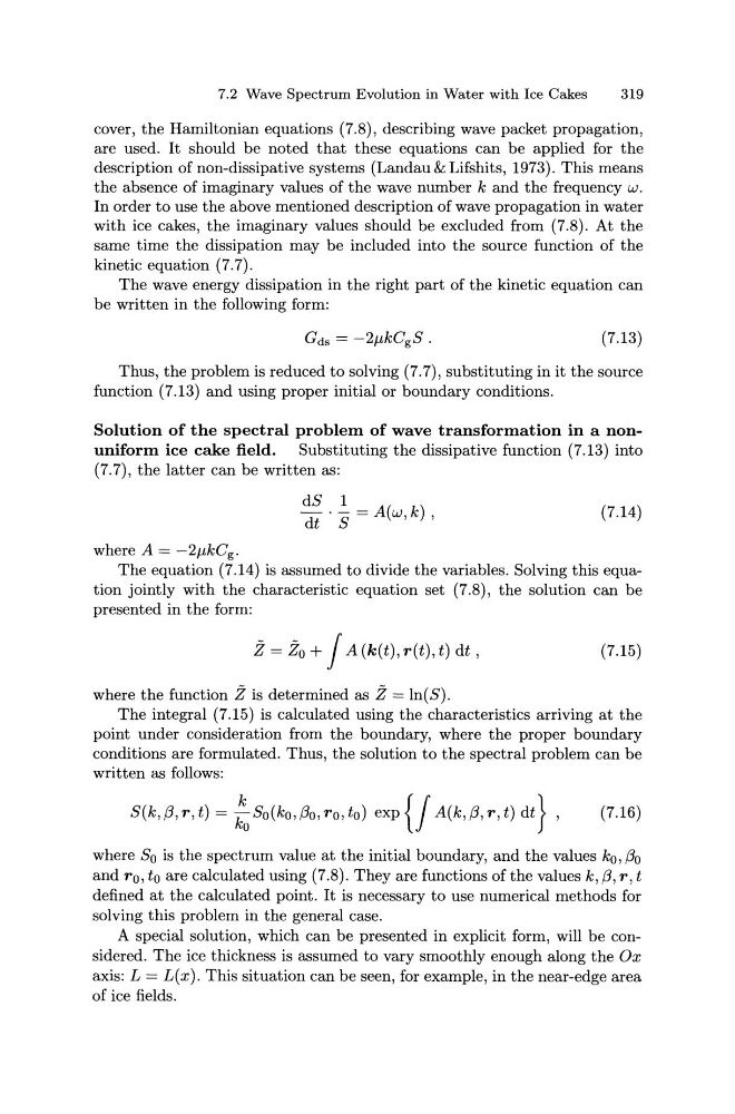
(7.13)
Thus, the problem is reduced to solving (7.7), substituting in it the source
function (7.13) and using proper initial or boundary conditions.
Solution of the spectral problem of wave transformation in a nonuniform ice cake field. Substituting the dissipative function (7.13) into
(7. 7), the latter can be written as:
dS 1
dt · S = A(w, k),
(7.14)
where A= -2p,kCg.
The equation (7.14) is assumed to divide the variables. Solving this equation jointly with the characteristic equation set (7.8), the solution can be
presented in the form:
Z = Zo + j A (k(t), r(t), t) dt,
(7.15)
where the function Z is determined as Z = ln(S).
The integral (7.15) is calculated using the characteristics arriving at the
point under consideration from the boundary, where the proper boundary
conditions are formulated. Thus, the solution to the spectral problem can be
written as follows:
S(k, {3, r, t) = : 0 So(ko, f3o, ro, to) exp { / A(k, {3, r, t) dt} ,
(7.16)
where So is the spectrum value at the initial boundary, and the values k0 , {3 0
and ro, to are calculated using (7.8). They are functions of the values k, {3, r, t
defined at the calculated point. It is necessary to use numerical methods for
solving this problem in the general case.
A special solution, which can be presented in explicit form, will be considered. The ice thickness is assumed to vary smoothly enough along the Ox
axis: L = L(x). This situation can be seen, for example, in the near-edge area
of ice fields.
319
cover, the Hamiltonian equations (7.8), describing wave packet propagation,
are used. It should be noted that these equations can be applied for the
description of non-dissipative systems (Landau & Lifshits, 1973). This means
the absence of imaginary values of the wave number k and the frequency w.
In order to use the above mentioned description of wave propagation in water
with ice cakes, the imaginary values should be excluded from (7.8). At the
same time the dissipation may be included into the source function of the
kinetic equation (7.7).
The wave energy dissipation in the right part of the kinetic equation can
be written in the following form:
(7.13)
Thus, the problem is reduced to solving (7.7), substituting in it the source
function (7.13) and using proper initial or boundary conditions.
Solution of the spectral problem of wave transformation in a nonuniform ice cake field. Substituting the dissipative function (7.13) into
(7. 7), the latter can be written as:
dS 1
dt · S = A(w, k),
(7.14)
where A= -2p,kCg.
The equation (7.14) is assumed to divide the variables. Solving this equation jointly with the characteristic equation set (7.8), the solution can be
presented in the form:
Z = Zo + j A (k(t), r(t), t) dt,
(7.15)
where the function Z is determined as Z = ln(S).
The integral (7.15) is calculated using the characteristics arriving at the
point under consideration from the boundary, where the proper boundary
conditions are formulated. Thus, the solution to the spectral problem can be
written as follows:
S(k, {3, r, t) = : 0 So(ko, f3o, ro, to) exp { / A(k, {3, r, t) dt} ,
(7.16)
where So is the spectrum value at the initial boundary, and the values k0 , {3 0
and ro, to are calculated using (7.8). They are functions of the values k, {3, r, t
defined at the calculated point. It is necessary to use numerical methods for
solving this problem in the general case.
A special solution, which can be presented in explicit form, will be considered. The ice thickness is assumed to vary smoothly enough along the Ox
axis: L = L(x). This situation can be seen, for example, in the near-edge area
of ice fields.