

OCEAN MODELS
83
K ij and an antisymmetric S ij part. With classical isotropic diffusion,
K ij is diagonal with mixing coefficient κ along the diagonal, and S ij is
zero. Taking into account the anisotropy of ocean motions requires a
different coefficient for horizontal and vertical mixing. More generally,
the symmetric tensor K ij can be diagonalized along principal mixing directions; in the ocean those are assumed to be along and across isopycnal
(isoneutral) directions respectively (see section 5.2). The corresponding
paramerization in the temperature and salinity equations for an ocean
model is called “isopycnal laplacian diffusion”, by contrast with horizontal diffusion.
One way to understand the antisymmetric part S ij is the following.
With eddy fluxes defined by (5) the equation for the resolved temperature T R includes the divergence of the eddy fluxes, with a contribution
from the antisymmetric tensor written as:
∇(−S ij
∂T R
∂x j
).
(6)
It is easily demonstrated that this term is identical to an advection of
T R by a velocity V ∗ with components defined by:
v
∗
i =
∂S ij
∂x j
.
(7)
As a consequense, in our idealized framework of a linear relationship
between eddy fluxes and mean gradients, parameterizations can be classified in three components: the vertical (cross isopycnal) and the lateral
(isopycnal) mixing associated with the symmetric tensor K ij , and the
advective eddy effect associated with S ij . Those three components will
be considered in turn in sections 3, 5 and 6 of this chapter. The interested reader will find a complete discussion of the mixing tensor (as well
as an alternative presentation using the notion of skew flux) in Griffies
(2004).
1.3
The diffusion equation
Parameterizations often assume a flux gradient relationship like (4),
and look like a diffusion. It is important to realize that the diffusion
equation has some unexpected properties when the mixing coefficient is
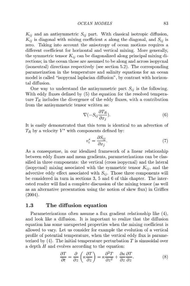
allowed to vary. Let us consider for example the evolution of a vertical
profile of potential temperature, when the vertical eddy flux is parameterized by (4). The initial temperature perturbation T is sinusoidal over
a depth H and evolves according to the equation:
∂T
∂t
=
∂
∂z
κ
∂T
∂z
= κ
∂ 2 T
∂z 2 +
∂κ
∂z
∂T
∂z
.
(8)
83
K ij and an antisymmetric S ij part. With classical isotropic diffusion,
K ij is diagonal with mixing coefficient κ along the diagonal, and S ij is
zero. Taking into account the anisotropy of ocean motions requires a
different coefficient for horizontal and vertical mixing. More generally,
the symmetric tensor K ij can be diagonalized along principal mixing directions; in the ocean those are assumed to be along and across isopycnal
(isoneutral) directions respectively (see section 5.2). The corresponding
paramerization in the temperature and salinity equations for an ocean
model is called “isopycnal laplacian diffusion”, by contrast with horizontal diffusion.
One way to understand the antisymmetric part S ij is the following.
With eddy fluxes defined by (5) the equation for the resolved temperature T R includes the divergence of the eddy fluxes, with a contribution
from the antisymmetric tensor written as:
∇(−S ij
∂T R
∂x j
).
(6)
It is easily demonstrated that this term is identical to an advection of
T R by a velocity V ∗ with components defined by:
v
∗
i =
∂S ij
∂x j
.
(7)
As a consequense, in our idealized framework of a linear relationship
between eddy fluxes and mean gradients, parameterizations can be classified in three components: the vertical (cross isopycnal) and the lateral
(isopycnal) mixing associated with the symmetric tensor K ij , and the
advective eddy effect associated with S ij . Those three components will
be considered in turn in sections 3, 5 and 6 of this chapter. The interested reader will find a complete discussion of the mixing tensor (as well
as an alternative presentation using the notion of skew flux) in Griffies
(2004).
1.3
The diffusion equation
Parameterizations often assume a flux gradient relationship like (4),
and look like a diffusion. It is important to realize that the diffusion
equation has some unexpected properties when the mixing coefficient is
allowed to vary. Let us consider for example the evolution of a vertical
profile of potential temperature, when the vertical eddy flux is parameterized by (4). The initial temperature perturbation T is sinusoidal over
a depth H and evolves according to the equation:
∂T
∂t
=
∂
∂z
κ
∂T
∂z
= κ
∂ 2 T
∂z 2 +
∂κ
∂z
∂T
∂z
.
(8)