

76
ANNE MARIE TREGUIER
−60
−50
−40
−30
−20
−10
0
10
20
30
−70
−60
−50
−40
−30
−20
−10
0
Longitude
Latitude
Sea surface height, ORCA2
0.1
0.2
−1.7
−1.8
− 0 .1
− 0 .2
− 1 .1
− 1
−0.3
−0.1
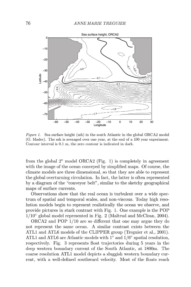
Figure 1. Sea surface height (ssh) in the south Atlantic in the global ORCA2 model
(G. Madec). The ssh is averaged over one year, at the end of a 100 year experiment.
Contour interval is 0.1 m, the zero contour is indicated in dark.
from the global 2 ◦ model ORCA2 (Fig. 1) is completely in agreement
with the image of the ocean conveyed by simplified maps. Of course, the
climate models are three dimensional, so that they are able to represent
the global overturning circulation. In fact, the latter is often represented
by a diagram of the “conveyor belt”, similar to the sketchy geographical
maps of surface currents.
Observations show that the real ocean is turbulent over a wide spectrum of spatial and temporal scales, and non-viscous. Today high resolution models begin to represent realistically the ocean we observe, and
provide pictures in stark contrast with Fig. 1. One example is the POP
1/10 ◦ global model represented in Fig. 2 (Maltrud and McClean, 2004).
ORCA2 and POP 1/10 are so different that one may argue they do
not represent the same ocean. A similar contrast exists between the
ATL1 and ATL6 models of the CLIPPER group (Treguier et al., 2001).
ATL1 and ATL6 are Atlantic models with 1 ◦ and 1/6 ◦ spatial resolution,
respectively. Fig. 3 represents float trajectories during 5 years in the
deep western boundary current of the South Atlantic, at 1800m. The
coarse resolution ATL1 model depicts a sluggish western boundary current, with a well-defined southward velocity. Most of the floats reach
ANNE MARIE TREGUIER
−60
−50
−40
−30
−20
−10
0
10
20
30
−70
−60
−50
−40
−30
−20
−10
0
Longitude
Latitude
Sea surface height, ORCA2
0.1
0.2
−1.7
−1.8
− 0 .1
− 0 .2
− 1 .1
− 1
−0.3
−0.1
Figure 1. Sea surface height (ssh) in the south Atlantic in the global ORCA2 model
(G. Madec). The ssh is averaged over one year, at the end of a 100 year experiment.
Contour interval is 0.1 m, the zero contour is indicated in dark.
from the global 2 ◦ model ORCA2 (Fig. 1) is completely in agreement
with the image of the ocean conveyed by simplified maps. Of course, the
climate models are three dimensional, so that they are able to represent
the global overturning circulation. In fact, the latter is often represented
by a diagram of the “conveyor belt”, similar to the sketchy geographical
maps of surface currents.
Observations show that the real ocean is turbulent over a wide spectrum of spatial and temporal scales, and non-viscous. Today high resolution models begin to represent realistically the ocean we observe, and
provide pictures in stark contrast with Fig. 1. One example is the POP
1/10 ◦ global model represented in Fig. 2 (Maltrud and McClean, 2004).
ORCA2 and POP 1/10 are so different that one may argue they do
not represent the same ocean. A similar contrast exists between the
ATL1 and ATL6 models of the CLIPPER group (Treguier et al., 2001).
ATL1 and ATL6 are Atlantic models with 1 ◦ and 1/6 ◦ spatial resolution,
respectively. Fig. 3 represents float trajectories during 5 years in the
deep western boundary current of the South Atlantic, at 1800m. The
coarse resolution ATL1 model depicts a sluggish western boundary current, with a well-defined southward velocity. Most of the floats reach