

559
The free surface and depth-integrated velocity boundary conditions use the
method of Flather (1976) with the external values specified by the
climatology plus tidal variability (harmonics M 2 , N 2 , S 2 , K 1 , O 1 , M 4 and M 6 )
from an ADCIRC model simulation of the western Atlantic (Luettich et al.
1992). Air-sea fluxes of momentum and heat were computed using bulk
formulae (Fairall et al. 1996) applied to the modeled sea surface temperature
and atmospheric marine boundary values (10-m wind, 2-m air temperature,
sea level pressure and relative humidity) and downward shortwave and longwave radiation from the 3-km resolution COAMPS forecast. Mellor-Yamada
(1982) mixing and quadratic bottom drag complete the model configuration.
During August-September of 2003, ocean forecasts were produced each
day as an aid to daily operations of the field program. Data from 72-hour
COAMPS forecasts that started each day at 0000 UTC and 1200 UTC were
delivered to Rutgers after the forecast completed, typically about 12 hours
after the start of the forecast cycle. The subsequent ROMS forecast,
initialized from the previous ocean model run, was therefore at best a 60hour forecast depending on the timeliness of the COAMPS data transfer,
which was sometimes delayed. Summary 3-hour interval forecast results
were posted on the web each day showing near surface currents and sea
temperature with the coincident COAMPS winds, plus a summary for each
forecast cycle of simulated Lagrangian float paths as a visualization the
pathways of lateral heat advection.
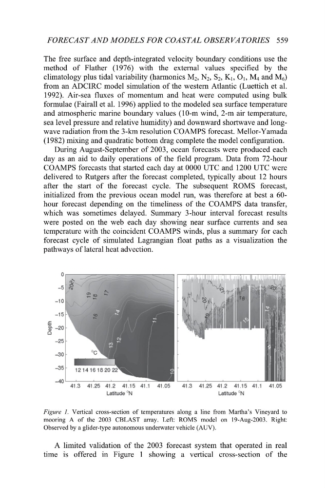
Figure 1. Vertical cross-section of temperatures along a line from Martha’s Vineyard to
mooring A of the 2003 CBLAST array. Left: ROMS model on 19-Aug-2003. Right:
Observed by a glider-type autonomous underwater vehicle (AUV).
A limited validation of the 2003 forecast system that operated in real
time is offered in Figure 1 showing a vertical cross-section of the
FORECAST AND MODELS FOR COASTAL OBSERVATORIES