

46
STEPHEN GRIFFIES
generalized vertical coordinate is given by the horizontal convergence of
mass per area onto that point. The transport is quasi-two-dimensional in
the sense that it is only a two-dimensional convergence that determines
the evolution. The tracer equation has an analogous interpretation. We
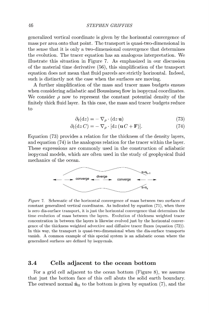
illustrate this situation in Figure 7. As emphasized in our discussion
of the material time derivative (56), this simplification of the transport
equation does not mean that fluid parcels are strictly horizontal. Indeed,
such is distinctly not the case when the surfaces are moving.
A further simplification of the mass and tracer mass budgets ensues
when considering adiabatic and Boussinesq flow in isopycnal coordinates.
We consider ρ now to represent the constant potential density of the
finitely thick fluid layer. In this case, the mass and tracer budgets reduce
to
∂ t (dz) = − ∇ ρ · (dz u)
(73)
∂ t (dz C) = − ∇ ρ · [dz (u C + F)].
(74)
Equation (73) provides a relation for the thickness of the density layers,
and equation (74) is the analogous relation for the tracer within the layer.
These expressions are commonly used in the construction of adiabatic
isopycnal models, which are often used in the study of geophysical fluid
mechanics of the ocean.
k−1
diverge
converge
converge
s=s k
s=s
Figure 7. Schematic of the horizontal convergence of mass between two surfaces of
constant generalized vertical coordinates. As indicated by equation (71), when there
is zero dia-surface transport, it is just the horizontal convergence that determines the
time evolution of mass between the layers. Evolution of thickness weighted tracer
concentration in between the layers is likewise evolved just by the horizontal convergence of the thickness weighted advective and diffusive tracer fluxes (equation (72)).
In this way, the transport is quasi-two-dimensional when the dia-surface transports
vanish. A common example of this special system is an adiabatic ocean where the
generalized surfaces are defined by isopycnals.
3.4
Cells adjacent to the ocean bottom
For a grid cell adjacent to the ocean bottom (Figure 8), we assume
that just the bottom face of this cell abuts the solid earth boundary.
The outward normal ˆ
n H to the bottom is given by equation (7), and the
STEPHEN GRIFFIES
generalized vertical coordinate is given by the horizontal convergence of
mass per area onto that point. The transport is quasi-two-dimensional in
the sense that it is only a two-dimensional convergence that determines
the evolution. The tracer equation has an analogous interpretation. We
illustrate this situation in Figure 7. As emphasized in our discussion
of the material time derivative (56), this simplification of the transport
equation does not mean that fluid parcels are strictly horizontal. Indeed,
such is distinctly not the case when the surfaces are moving.
A further simplification of the mass and tracer mass budgets ensues
when considering adiabatic and Boussinesq flow in isopycnal coordinates.
We consider ρ now to represent the constant potential density of the
finitely thick fluid layer. In this case, the mass and tracer budgets reduce
to
∂ t (dz) = − ∇ ρ · (dz u)
(73)
∂ t (dz C) = − ∇ ρ · [dz (u C + F)].
(74)
Equation (73) provides a relation for the thickness of the density layers,
and equation (74) is the analogous relation for the tracer within the layer.
These expressions are commonly used in the construction of adiabatic
isopycnal models, which are often used in the study of geophysical fluid
mechanics of the ocean.
k−1
diverge
converge
converge
s=s k
s=s
Figure 7. Schematic of the horizontal convergence of mass between two surfaces of
constant generalized vertical coordinates. As indicated by equation (71), when there
is zero dia-surface transport, it is just the horizontal convergence that determines the
time evolution of mass between the layers. Evolution of thickness weighted tracer
concentration in between the layers is likewise evolved just by the horizontal convergence of the thickness weighted advective and diffusive tracer fluxes (equation (72)).
In this way, the transport is quasi-two-dimensional when the dia-surface transports
vanish. A common example of this special system is an adiabatic ocean where the
generalized surfaces are defined by isopycnals.
3.4
Cells adjacent to the ocean bottom
For a grid cell adjacent to the ocean bottom (Figure 8), we assume
that just the bottom face of this cell abuts the solid earth boundary.
The outward normal ˆ
n H to the bottom is given by equation (7), and the