

SOME OCEAN MODEL FUNDAMENTALS
43
used in the model. On the right hand side, s(') represents a tracer
source with units of tracer concentration per time. As seen in Section
2.5, dA(,). n - (v - vref) measures the volume per time of fluid penetrating
the domain boundary at a point.
The tracer flux J arises from subgrid scale transport, such as diffusion
and/or unresolved advection. This flux is assumed to vanish when the
tracer concentration is uniform, in which case the tracer budget (57)
reduces to a mass budget. In addition to the tracer flux, it is convenient
to define the tracer concentration flux F via
where the dimensions of F are velocity x tracer concentration.
3.2
Budget for an interior grid cell
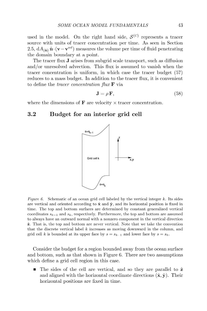
Figure 6. Schematic of an ocean grid cell labeled by the vertical integer Ic. Its sides
are vertical and oriented according to P and 9, and its horizontal position is fmed in
time. The top and bottom surfaces are determined by constant generalized vertical
coordinates s k - 1 and s k , respectively. Furthermore, the top and bottom are assumed
to always have an outward normal with a nonzero component in the vertical direction
%. That is, the top and bottom are never vertical. Note that we take the convention
that the discrete vertical label Ic increases as moving downward in the column, and
grid cell k is bounded at its upper face by s = s k - 1 and lower face by s = s k .
Consider the budget for a region bounded away from the ocean surface
and bottom, such as that shown in Figure 6. There are two assumptions
which define a grid cell region in this case.
The sides of the cell are vertical, and so they are parallel to B
and aligned with the horizontal coordinate directions (k,?). Their
horizontal positions are fixed in time.
43
used in the model. On the right hand side, s(') represents a tracer
source with units of tracer concentration per time. As seen in Section
2.5, dA(,). n - (v - vref) measures the volume per time of fluid penetrating
the domain boundary at a point.
The tracer flux J arises from subgrid scale transport, such as diffusion
and/or unresolved advection. This flux is assumed to vanish when the
tracer concentration is uniform, in which case the tracer budget (57)
reduces to a mass budget. In addition to the tracer flux, it is convenient
to define the tracer concentration flux F via
where the dimensions of F are velocity x tracer concentration.
3.2
Budget for an interior grid cell
Figure 6. Schematic of an ocean grid cell labeled by the vertical integer Ic. Its sides
are vertical and oriented according to P and 9, and its horizontal position is fmed in
time. The top and bottom surfaces are determined by constant generalized vertical
coordinates s k - 1 and s k , respectively. Furthermore, the top and bottom are assumed
to always have an outward normal with a nonzero component in the vertical direction
%. That is, the top and bottom are never vertical. Note that we take the convention
that the discrete vertical label Ic increases as moving downward in the column, and
grid cell k is bounded at its upper face by s = s k - 1 and lower face by s = s k .
Consider the budget for a region bounded away from the ocean surface
and bottom, such as that shown in Figure 6. There are two assumptions
which define a grid cell region in this case.
The sides of the cell are vertical, and so they are parallel to B
and aligned with the horizontal coordinate directions (k,?). Their
horizontal positions are fixed in time.