

354
FLORENCE RABIER
J true (x)= J b /s b + J o /s o
(15)
is the cost function using « true » matrices.
Let x a be the minimizer of this cost function, then, following Talagrand
(1999)
E(2J o (x a )/s o )=Tr (I –HK)
(16)
E(2J b (x a )/sb)=Tr (KH)
(17)
yielding the following condition for the tuning coefficients
s o = 2J o (x a )/ Tr (I –HK)
(18)
s b = 2J b (x a )/ Tr (KH)
(19)
As K depends on s o and s b , this is a fixed-point relation, and a fixed point
algorithm can be used to estimate the tuning coefficients. The denominator
of those expressions can be computed using Girard’s method, which is also
used to compute the DFS.
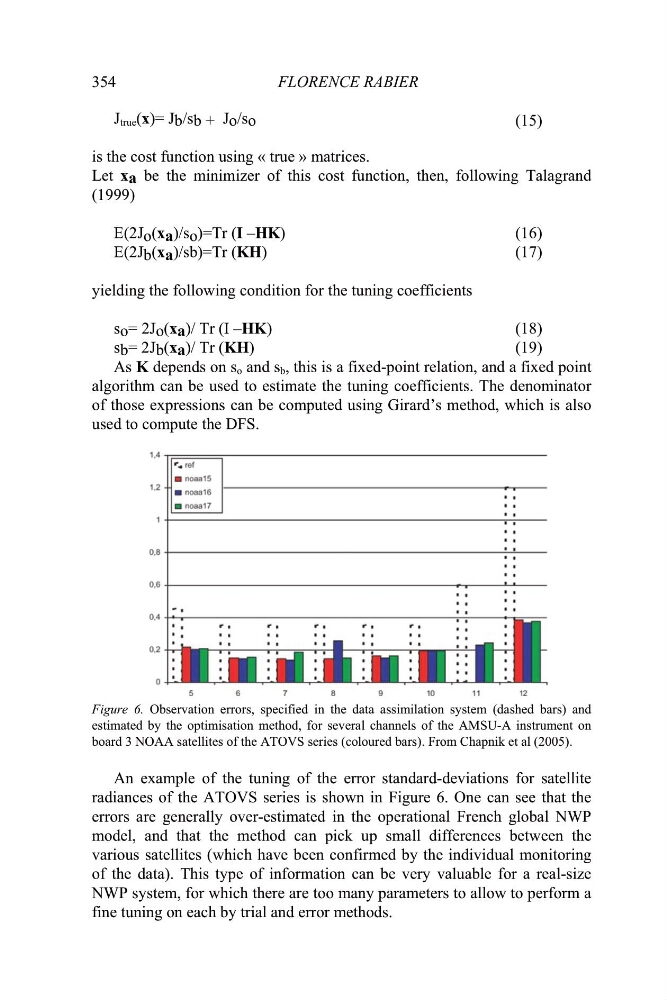
Figure 6. Observation errors, specified in the data assimilation system (dashed bars) and
estimated by the optimisation method, for several channels of the AMSU-A instrument on
board 3 NOAA satellites of the ATOVS series (coloured bars). From Chapnik et al (2005).
An example of the tuning of the error standard-deviations for satellite
radiances of the ATOVS series is shown in Figure 6. One can see that the
errors are generally over-estimated in the operational French global NWP
model, and that the method can pick up small differences between the
various satellites (which have been confirmed by the individual monitoring
of the data). This type of information can be very valuable for a real-size
NWP system, for which there are too many parameters to allow to perform a
fine tuning on each by trial and error methods.
FLORENCE RABIER
J true (x)= J b /s b + J o /s o
(15)
is the cost function using « true » matrices.
Let x a be the minimizer of this cost function, then, following Talagrand
(1999)
E(2J o (x a )/s o )=Tr (I –HK)
(16)
E(2J b (x a )/sb)=Tr (KH)
(17)
yielding the following condition for the tuning coefficients
s o = 2J o (x a )/ Tr (I –HK)
(18)
s b = 2J b (x a )/ Tr (KH)
(19)
As K depends on s o and s b , this is a fixed-point relation, and a fixed point
algorithm can be used to estimate the tuning coefficients. The denominator
of those expressions can be computed using Girard’s method, which is also
used to compute the DFS.
Figure 6. Observation errors, specified in the data assimilation system (dashed bars) and
estimated by the optimisation method, for several channels of the AMSU-A instrument on
board 3 NOAA satellites of the ATOVS series (coloured bars). From Chapnik et al (2005).
An example of the tuning of the error standard-deviations for satellite
radiances of the ATOVS series is shown in Figure 6. One can see that the
errors are generally over-estimated in the operational French global NWP
model, and that the method can pick up small differences between the
various satellites (which have been confirmed by the individual monitoring
of the data). This type of information can be very valuable for a real-size
NWP system, for which there are too many parameters to allow to perform a
fine tuning on each by trial and error methods.