

METEOROLOGICAL DATA PERSPECTIVE
353
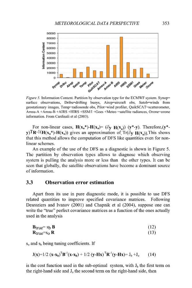
Figure 5. Information Content. Partition by observation type for the ECMWF system. Synop=
surface observations, Dribu=drifting buoys, Airep=aircraft obs, Satob=winds from
geostationary images, Temp=radiosonde obs, Pilot=wind profiler, QuikSCAT=scatterometer,
Amsu-A +Amsu-B +AIRS +HIRS +SSM/I +Goes +Meteo =satellite radiances, Ozone=ozone
information. From Cardinali et al (2003).
For non-linear cases, H(x a *)-H(x a )= ( y H( x a ) ) (y*-y). Therefore,(y*y) T R -1( H(x a *)-H(x a )) gives an approximation of Ҟ Tr( y H( x a )). This shows
that this method allows the computation of DFS like quantities even for nonlinear schemes.
An example of the use of the DFS as a diagnostic is shown in Figure 5.
The partition by observation types allows to diagnose which observing
system is pulling the analysis more or less than the other types. It can be
seen that globally, the satellite observations have become a dominant source
of information.
3.3
Observation error estimation
Apart from its use in pure diagnostic mode, it is possible to use DFS
related quantities to improve specified covariance matrices. Following
Desroziers and Ivanov (2001) and Chapnik et al (2004), suppose one can
write the “true” perfect covariance matrices as a function of the ones actually
used in the analysis
B true = s b B
(12)
R true =s o R
(13)
s o and s b being tuning coefficients. If
J(x)=1/2 (x-x b )
T
B
-1 (x-x b ) + 1/2 (y-Hx)
T
R
-1 (y-Hx)= J b +J o
(14)
is the cost function used in the sub-optimal system, with J b the first term on
the right-hand side and J o the second term on the right-hand side, then
353
Figure 5. Information Content. Partition by observation type for the ECMWF system. Synop=
surface observations, Dribu=drifting buoys, Airep=aircraft obs, Satob=winds from
geostationary images, Temp=radiosonde obs, Pilot=wind profiler, QuikSCAT=scatterometer,
Amsu-A +Amsu-B +AIRS +HIRS +SSM/I +Goes +Meteo =satellite radiances, Ozone=ozone
information. From Cardinali et al (2003).
For non-linear cases, H(x a *)-H(x a )= ( y H( x a ) ) (y*-y). Therefore,(y*y) T R -1( H(x a *)-H(x a )) gives an approximation of Ҟ Tr( y H( x a )). This shows
that this method allows the computation of DFS like quantities even for nonlinear schemes.
An example of the use of the DFS as a diagnostic is shown in Figure 5.
The partition by observation types allows to diagnose which observing
system is pulling the analysis more or less than the other types. It can be
seen that globally, the satellite observations have become a dominant source
of information.
3.3
Observation error estimation
Apart from its use in pure diagnostic mode, it is possible to use DFS
related quantities to improve specified covariance matrices. Following
Desroziers and Ivanov (2001) and Chapnik et al (2004), suppose one can
write the “true” perfect covariance matrices as a function of the ones actually
used in the analysis
B true = s b B
(12)
R true =s o R
(13)
s o and s b being tuning coefficients. If
J(x)=1/2 (x-x b )
T
B
-1 (x-x b ) + 1/2 (y-Hx)
T
R
-1 (y-Hx)= J b +J o
(14)
is the cost function used in the sub-optimal system, with J b the first term on
the right-hand side and J o the second term on the right-hand side, then