

300
PIERRE BRASSEUR
a series of separate smaller calculations using the partitioned Kalman
filter and smoother proposed by Fukumori [2002]. The objective of the
partition is to make global eddy-resolving data assimilation problems
computationally viable. In their example, the reduced state consists of
perturbations of the barotropic mode and the first five baroclinic modes
defined in eight overlapping cells covering the globe.
6.3
Stochastic vs. deterministic filters
In a low-rank filter like SEEK, the error directions are determined at
the initialization step and their evolution can be anticipated in a deterministic way. As these filters do not require any further randomization,
they are termed deterministic filters in contrast to the EnKF which can
be considered as a stochastic filter because ramdomization has to be
repeated at each assimilation cycle.
Evensen [2003] reviews the theoretical formulation and practical implementation of the EnKF. The EnKF was introduced to avoid the occurrence of instabilities found with the Extended KF due to the non-linear
evolution of the probability density functions [Evensen 1994]. However,
the EnKF only solves half of the non-linearity problems because it still
combines the model prediction and the data by using only the first
two moments of the pdfs, assuming that the distributions are nearly
Gaussian. The non-linear analysis equations would be more di!cult to
use in practical applications, as discussed by Evensen and van Leeuwen
[2000].
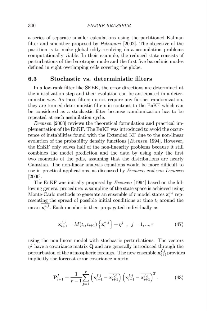
The EnKF was initially proposed by Evensen [1994] based on the following general procedure: a sampling of the state space is achieved using
Monte-Carlo methods to generate an ensemble of r model states x
a,j
i representing the spread of possible initial conditions at time t i around the
mean x
a,j
i . Each member is then propagated individually as
x
f,j
i+1 = M(t i , t i+1 )
q
x
a,j
i
r
+
j , j = 1, ..., r
(47)
using the non-linear model with stochastic perturbations. The vectors
j have a covariance matrix Q and are generally introduced through the
perturbation of the atmospheric forcings. The new ensemble x
f,j
i+1 provides
implicitly the forecast error covariance matrix
P
f
i+1 =
1
r 1
r
[
j=1
x
f,j
i+1 x
f,j
i+1
x
f,j
i+1 x
f,j
i+1
T
.
(48)
PIERRE BRASSEUR
a series of separate smaller calculations using the partitioned Kalman
filter and smoother proposed by Fukumori [2002]. The objective of the
partition is to make global eddy-resolving data assimilation problems
computationally viable. In their example, the reduced state consists of
perturbations of the barotropic mode and the first five baroclinic modes
defined in eight overlapping cells covering the globe.
6.3
Stochastic vs. deterministic filters
In a low-rank filter like SEEK, the error directions are determined at
the initialization step and their evolution can be anticipated in a deterministic way. As these filters do not require any further randomization,
they are termed deterministic filters in contrast to the EnKF which can
be considered as a stochastic filter because ramdomization has to be
repeated at each assimilation cycle.
Evensen [2003] reviews the theoretical formulation and practical implementation of the EnKF. The EnKF was introduced to avoid the occurrence of instabilities found with the Extended KF due to the non-linear
evolution of the probability density functions [Evensen 1994]. However,
the EnKF only solves half of the non-linearity problems because it still
combines the model prediction and the data by using only the first
two moments of the pdfs, assuming that the distributions are nearly
Gaussian. The non-linear analysis equations would be more di!cult to
use in practical applications, as discussed by Evensen and van Leeuwen
[2000].
The EnKF was initially proposed by Evensen [1994] based on the following general procedure: a sampling of the state space is achieved using
Monte-Carlo methods to generate an ensemble of r model states x
a,j
i representing the spread of possible initial conditions at time t i around the
mean x
a,j
i . Each member is then propagated individually as
x
f,j
i+1 = M(t i , t i+1 )
q
x
a,j
i
r
+
j , j = 1, ..., r
(47)
using the non-linear model with stochastic perturbations. The vectors
j have a covariance matrix Q and are generally introduced through the
perturbation of the atmospheric forcings. The new ensemble x
f,j
i+1 provides
implicitly the forecast error covariance matrix
P
f
i+1 =
1
r 1
r
[
j=1
x
f,j
i+1 x
f,j
i+1
x
f,j
i+1 x
f,j
i+1
T
.
(48)