

284
PIERRE BRASSEUR
for simplicity, so that y is a scalar ( p = 1) and H is a single-row vector
of the form
H = [0, ..., 0, 1, 0, ..., 0]
(23)
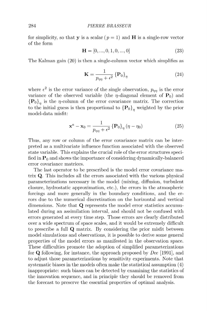
The Kalman gain (20) is then a single-column vector which simplifies as
K =
1
p + 2 {P 0 }
(24)
where
2 is the error variance of the single observation, p is the error
variance of the observed variable (the -diagonal element of P 0 ) and
{P 0 } is the -column of the error covariance matrix. The correction
to the initial guess is then proportional to {P 0 } weighted by the prior
model-data misfit:
x
a x 0 =
1
p + 2 {P 0 } ( 0 )
(25)
Thus, any row or column of the error covariance matrix can be interpreted as a multivariate influence function associated with the observed
state variable. This explains the crucial role of the error structures specified in P 0 and shows the importance of considering dynamically-balanced
error covariance matrices.
The last operator to be prescribed is the model error covariance matrix Q. This includes all the errors associated with the various physical
parameterizations necessary in the model (mixing, diusion, turbulent
closure, hydrostatic approximation, etc.), the errors in the atmospheric
forcings and more generally in the boundary conditions, and the errors due to the numerical discretization on the horizontal and vertical
dimensions. Note that Q represents the model error statistics accumulated during an assimilation interval, and should not be confused with
errors generated at every time step. Those errors are clearly distributed
over a wide spectrum of space scales, and it would be extremely di!cult
to prescribe a full Q matrix. By considering the prior misfit between
model simulations and observations, it is possible to derive some general
properties of the model errors as manifested in the observation space.
These di!culties promote the adoption of simplified parameterizations
for Q following, for instance, the approach proposed by Dee [1991], and
to adjust those parameterizations by sensitivity experiments. Note that
systematic biases in the models often make the statistical assumption (4)
inappropriate: such biases can be detected by examining the statistics of
the innovation sequence, and in principle they should be removed from
the forecast to preserve the essential properties of optimal analysis.
PIERRE BRASSEUR
for simplicity, so that y is a scalar ( p = 1) and H is a single-row vector
of the form
H = [0, ..., 0, 1, 0, ..., 0]
(23)
The Kalman gain (20) is then a single-column vector which simplifies as
K =
1
p + 2 {P 0 }
(24)
where
2 is the error variance of the single observation, p is the error
variance of the observed variable (the -diagonal element of P 0 ) and
{P 0 } is the -column of the error covariance matrix. The correction
to the initial guess is then proportional to {P 0 } weighted by the prior
model-data misfit:
x
a x 0 =
1
p + 2 {P 0 } ( 0 )
(25)
Thus, any row or column of the error covariance matrix can be interpreted as a multivariate influence function associated with the observed
state variable. This explains the crucial role of the error structures specified in P 0 and shows the importance of considering dynamically-balanced
error covariance matrices.
The last operator to be prescribed is the model error covariance matrix Q. This includes all the errors associated with the various physical
parameterizations necessary in the model (mixing, diusion, turbulent
closure, hydrostatic approximation, etc.), the errors in the atmospheric
forcings and more generally in the boundary conditions, and the errors due to the numerical discretization on the horizontal and vertical
dimensions. Note that Q represents the model error statistics accumulated during an assimilation interval, and should not be confused with
errors generated at every time step. Those errors are clearly distributed
over a wide spectrum of space scales, and it would be extremely di!cult
to prescribe a full Q matrix. By considering the prior misfit between
model simulations and observations, it is possible to derive some general
properties of the model errors as manifested in the observation space.
These di!culties promote the adoption of simplified parameterizations
for Q following, for instance, the approach proposed by Dee [1991], and
to adjust those parameterizations by sensitivity experiments. Note that
systematic biases in the models often make the statistical assumption (4)
inappropriate: such biases can be detected by examining the statistics of
the innovation sequence, and in principle they should be removed from
the forecast to preserve the essential properties of optimal analysis.