

283
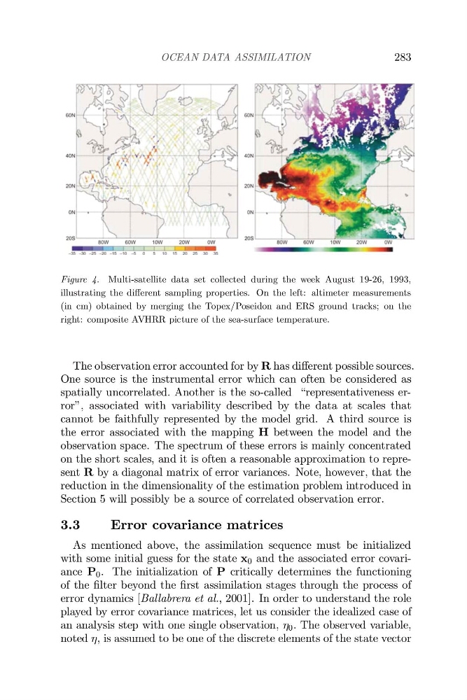
Figure 4. Multi-satellite data set collected during the week August 19-26, 1993,
illustrating the dierent sampling properties. On the left: altimeter measurements
(in cm) obtained by merging the Topex/Poseidon and ERS ground tracks; on the
right: composite AVHRR picture of the sea-surface temperature.
The observation error accounted for by R has dierent possible sources.
One source is the instrumental error which can often be considered as
spatially uncorrelated. Another is the so-called “representativeness error”, associated with variability described by the data at scales that
cannot be faithfully represented by the model grid. A third source is
the error associated with the mapping H between the model and the
observation space. The spectrum of these errors is mainly concentrated
on the short scales, and it is often a reasonable approximation to represent R by a diagonal matrix of error variances. Note, however, that the
reduction in the dimensionality of the estimation problem introduced in
Section 5 will possibly be a source of correlated observation error.
3.3
Error covariance matrices
As mentioned above, the assimilation sequence must be initialized
with some initial guess for the state x 0 and the associated error covariance P 0 . The initialization of P critically determines the functioning
of the filter beyond the first assimilation stages through the process of
error dynamics [Ballabrera et al., 2001]. In order to understand the role
played by error covariance matrices, let us consider the idealized case of
an analysis step with one single observation, 0 . The observed variable,
noted , is assumed to be one of the discrete elements of the state vector
OCEAN DATA ASSIMILATION
Figure 4. Multi-satellite data set collected during the week August 19-26, 1993,
illustrating the dierent sampling properties. On the left: altimeter measurements
(in cm) obtained by merging the Topex/Poseidon and ERS ground tracks; on the
right: composite AVHRR picture of the sea-surface temperature.
The observation error accounted for by R has dierent possible sources.
One source is the instrumental error which can often be considered as
spatially uncorrelated. Another is the so-called “representativeness error”, associated with variability described by the data at scales that
cannot be faithfully represented by the model grid. A third source is
the error associated with the mapping H between the model and the
observation space. The spectrum of these errors is mainly concentrated
on the short scales, and it is often a reasonable approximation to represent R by a diagonal matrix of error variances. Note, however, that the
reduction in the dimensionality of the estimation problem introduced in
Section 5 will possibly be a source of correlated observation error.
3.3
Error covariance matrices
As mentioned above, the assimilation sequence must be initialized
with some initial guess for the state x 0 and the associated error covariance P 0 . The initialization of P critically determines the functioning
of the filter beyond the first assimilation stages through the process of
error dynamics [Ballabrera et al., 2001]. In order to understand the role
played by error covariance matrices, let us consider the idealized case of
an analysis step with one single observation, 0 . The observed variable,
noted , is assumed to be one of the discrete elements of the state vector
OCEAN DATA ASSIMILATION