

OCEAN DATA ASSIMILATION
275
statistical assumptions are quite crude approximations of the actual error
distributions (in particular, a bias in the model is very common), but
they are very convenient in deriving a baseline of optimal estimation. A
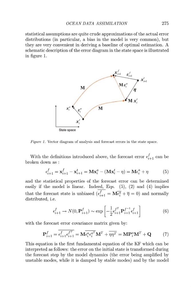
schematic description of the error diagram in the state space is illustrated
in figure 1.
Figure 1. Vector diagram of analysis and forecast errors in the state space.
With the definitions introduced above, the forecast error
f
i+1 can be
broken down as :
f
i+1 = x
f
i+1 x
t
i+1 = Mx
a
i (Mx
t
i ) = M
a
i +
(5)
and the statistical properties of the forecast error can be determined
easily if the model is linear. Indeed, Eqs. (5), (2) and (4) implies
that the forecast state is unbiased (
f
i+1 = M a
i + = 0) and normally
distributed, i.e.
f
i+1 $ N (0, P
f
i+1 ) exp
1
2
f T
i+1 P
f 31
i+1
f
i+1
(6)
with the forecast error covariance matrix given by:
P
f
i+1 =
f
i+1
f T
i+1 = M a
i a T
i M
T
+ T = MP
a
i M
T
+ Q
(7)
This equation is the first fundamental equation of the KF which can be
interpreted as follows: the error on the initial state is transformed during
the forecast step by the model dynamics (the error being amplified by
unstable modes, while it is damped by stable modes) and by the model
275
statistical assumptions are quite crude approximations of the actual error
distributions (in particular, a bias in the model is very common), but
they are very convenient in deriving a baseline of optimal estimation. A
schematic description of the error diagram in the state space is illustrated
in figure 1.
Figure 1. Vector diagram of analysis and forecast errors in the state space.
With the definitions introduced above, the forecast error
f
i+1 can be
broken down as :
f
i+1 = x
f
i+1 x
t
i+1 = Mx
a
i (Mx
t
i ) = M
a
i +
(5)
and the statistical properties of the forecast error can be determined
easily if the model is linear. Indeed, Eqs. (5), (2) and (4) implies
that the forecast state is unbiased (
f
i+1 = M a
i + = 0) and normally
distributed, i.e.
f
i+1 $ N (0, P
f
i+1 ) exp
1
2
f T
i+1 P
f 31
i+1
f
i+1
(6)
with the forecast error covariance matrix given by:
P
f
i+1 =
f
i+1
f T
i+1 = M a
i a T
i M
T
+ T = MP
a
i M
T
+ Q
(7)
This equation is the first fundamental equation of the KF which can be
interpreted as follows: the error on the initial state is transformed during
the forecast step by the model dynamics (the error being amplified by
unstable modes, while it is damped by stable modes) and by the model