

248
WILLIAM B. LARGE
it is necessary to treat stable and unstable heat fluxes separately. The
positive offset is consistent with an unbounded transfer coefficient (slope)
as wind speed approaches zero, but the flux, as in the case of (8), should
diminish. This behavior can also be achieved by combining (29) and
(31), then using fluxes to compute the roughness lengths from
κ
ln(10m/z θ )
=
1
√
C DN
u ∗ θ ∗
θ N U N
;
(39)
κ
ln(10m/z q )
=
1
√
C DN
u ∗ q ∗
q N U N
.
(40)
Empirically, (39) is found to average about 0.0180 in stable conditions
and 0.0327 in unstable, while a typical value of (40) is about 0.0346.
There is relatively little scatter in these values, because of the observed
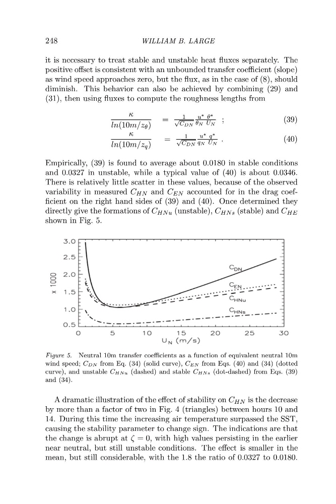
variability in measured C HN and C EN accounted for in the drag coefficient on the right hand sides of (39) and (40). Once determined they
directly give the formations of C HNu (unstable), C HNs (stable) and C HE
shown in Fig. 5.
Figure 5. Neutral 10m transfer coefficients as a function of equivalent neutral 10m
wind speed; CDN from Eq. (34) (solid curve), CEN from Eqs. (40) and (34) (dotted
curve), and unstable CHNu (dashed) and stable CHNs (dot-dashed) from Eqs. (39)
and (34).
A dramatic illustration of the effect of stability on C HN is the decrease
by more than a factor of two in Fig. 4 (triangles) between hours 10 and
14. During this time the increasing air temperature surpassed the SST,
causing the stability parameter to change sign. The indications are that
the change is abrupt at ζ = 0, with high values persisting in the earlier
near neutral, but still unstable conditions. The effect is smaller in the
mean, but still considerable, with the 1.8 the ratio of 0.0327 to 0.0180.
WILLIAM B. LARGE
it is necessary to treat stable and unstable heat fluxes separately. The
positive offset is consistent with an unbounded transfer coefficient (slope)
as wind speed approaches zero, but the flux, as in the case of (8), should
diminish. This behavior can also be achieved by combining (29) and
(31), then using fluxes to compute the roughness lengths from
κ
ln(10m/z θ )
=
1
√
C DN
u ∗ θ ∗
θ N U N
;
(39)
κ
ln(10m/z q )
=
1
√
C DN
u ∗ q ∗
q N U N
.
(40)
Empirically, (39) is found to average about 0.0180 in stable conditions
and 0.0327 in unstable, while a typical value of (40) is about 0.0346.
There is relatively little scatter in these values, because of the observed
variability in measured C HN and C EN accounted for in the drag coefficient on the right hand sides of (39) and (40). Once determined they
directly give the formations of C HNu (unstable), C HNs (stable) and C HE
shown in Fig. 5.
Figure 5. Neutral 10m transfer coefficients as a function of equivalent neutral 10m
wind speed; CDN from Eq. (34) (solid curve), CEN from Eqs. (40) and (34) (dotted
curve), and unstable CHNu (dashed) and stable CHNs (dot-dashed) from Eqs. (39)
and (34).
A dramatic illustration of the effect of stability on C HN is the decrease
by more than a factor of two in Fig. 4 (triangles) between hours 10 and
14. During this time the increasing air temperature surpassed the SST,
causing the stability parameter to change sign. The indications are that
the change is abrupt at ζ = 0, with high values persisting in the earlier
near neutral, but still unstable conditions. The effect is smaller in the
mean, but still considerable, with the 1.8 the ratio of 0.0327 to 0.0180.