

SURFA CE FL UXES
241
downstream radian wavenumber, Ic, by Taylor's frozen turbulence hypothesis, Ic = 2xflU. The time average of a vertical flux of property X
at a point is the integral over frequency, f , of the cospectrum, @,,(f), of
the property fluctuations, x, and the vertical velocity, w. Similarly, the
spatial average at a point in time is the integral of the cospectrum over
k. In practice, the eddies occupy a finite range of wavenumber space, say
kl to Ic2, and hence frequency space, say fi to f2, so the fluxes become
I 1 1 1 1 1 1 1 ~
I 1 1 1 1 1 1 1 ~
I 1 1 1 1 1 1 1 ~
I I 1 1 1 1 1 1 ~
I 1 1 1 1 1 1 1 ~
I I I I I
/ \
1'
', STABLE
UNSTABLE
I
\
I
\
I
\
I
\
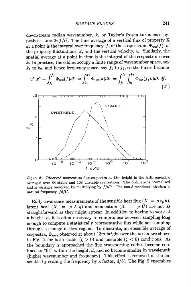
Figure 2. Observed momentum flux cospectra at 13m height in the ABL ensemble
averaged over 88 stable and 108 unstable realizations. The ordinate is normalized
and is variance preserved by multiplying by flu*'. The non-dimensional abscissa is
natural frequency, f d/U.
Eddy covariance measurements of the sensible heat flux ( X = p cp 69,
latent heat ( X = p A q) and momentum ( X = p U) are not as
straightforward as they might appear. In addition to having to work at
a height, d, it is often necessary to compromise between sampling long
enough to compute a statistically representative flux while not sampling
through a change in flow regime. To illustrate, an ensemble average of
cospectra, a, , , observed at about 13m height over the ocean are shown
in Fig. 2 for both stable (( > 0) and unstable (( < 0) conditions. As
the boundary is approached the flux transporting eddies become confined to "fit" within the height, d, and so become smaller in wavelength
(higher wavenumber and frequency). This effect is removed in the ensemble by scaling the frequency by a factor, dlU. The Fig. 2 ensembles
241
downstream radian wavenumber, Ic, by Taylor's frozen turbulence hypothesis, Ic = 2xflU. The time average of a vertical flux of property X
at a point is the integral over frequency, f , of the cospectrum, @,,(f), of
the property fluctuations, x, and the vertical velocity, w. Similarly, the
spatial average at a point in time is the integral of the cospectrum over
k. In practice, the eddies occupy a finite range of wavenumber space, say
kl to Ic2, and hence frequency space, say fi to f2, so the fluxes become
I 1 1 1 1 1 1 1 ~
I 1 1 1 1 1 1 1 ~
I 1 1 1 1 1 1 1 ~
I I 1 1 1 1 1 1 ~
I 1 1 1 1 1 1 1 ~
I I I I I
/ \
1'
', STABLE
UNSTABLE
I
\
I
\
I
\
I
\
Figure 2. Observed momentum flux cospectra at 13m height in the ABL ensemble
averaged over 88 stable and 108 unstable realizations. The ordinate is normalized
and is variance preserved by multiplying by flu*'. The non-dimensional abscissa is
natural frequency, f d/U.
Eddy covariance measurements of the sensible heat flux ( X = p cp 69,
latent heat ( X = p A q) and momentum ( X = p U) are not as
straightforward as they might appear. In addition to having to work at
a height, d, it is often necessary to compromise between sampling long
enough to compute a statistically representative flux while not sampling
through a change in flow regime. To illustrate, an ensemble average of
cospectra, a, , , observed at about 13m height over the ocean are shown
in Fig. 2 for both stable (( > 0) and unstable (( < 0) conditions. As
the boundary is approached the flux transporting eddies become confined to "fit" within the height, d, and so become smaller in wavelength
(higher wavenumber and frequency). This effect is removed in the ensemble by scaling the frequency by a factor, dlU. The Fig. 2 ensembles