

158
IAN ROBINSON
about 1340 km where atmospheric drag is minimal, the height of the satellite
in orbit, H sat , can now be predicted to a precision of 2 cm (Tapley et al.,
1994) using a combination of laser and microwave tracking devices and an
orbit model using precise gravity fields. The tidal contribution has been
evaluated along the repeat orbit track by tidal analysis of the altimeter record
spanning several years (Le Provost, 2001). Because the tidal frequencies are
very precisely known the response to each constituent can be evaluated to an
accuracy better than 2 cm in the open ocean, even though the sampling
interval of about 10 days is longer than most of the tidal periods. This is
only possible when the precise period of the repeat cycle is chosen to avoid
any serious aliasing with one of the major tidal constituents. For this reason
a sun-synchronous orbit, which aliases the S 2 (solar semidiurnal) tidal signal,
should not be used. Over shelf seas where tides are very high and can vary
rapidly over short distances it is not so easy to remove the tides and so the
estimate of dynamic height is less accurate. The atmospheric pressure
correction is based on the output of atmospheric circulation models.
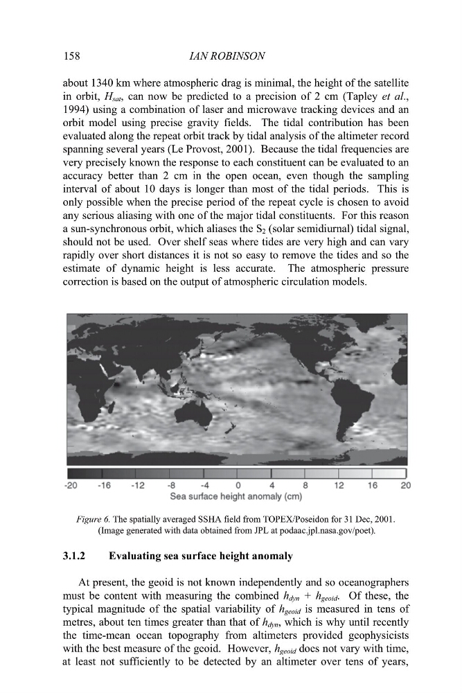
Figure 6. The spatially averaged SSHA field from TOPEX/Poseidon for 31 Dec, 2001.
(Image generated with data obtained from JPL at podaac.jpl.nasa.gov/poet)
3.1.2
Evaluating sea surface height anomaly
At present, the geoid is not known independently and so oceanographers
must be content with measuring the combined h dyn + h geoid . Of these, the
typical magnitude of the spatial variability of h geoid is measured in tens of
metres, about ten times greater than that of h dyn , which is why until recently
the time-mean ocean topography from altimeters provided geophysicists
with the best measure of the geoid. However, h geoid does not vary with time,
at least not sufficiently to be detected by an altimeter over tens of years,
.
IAN ROBINSON
about 1340 km where atmospheric drag is minimal, the height of the satellite
in orbit, H sat , can now be predicted to a precision of 2 cm (Tapley et al.,
1994) using a combination of laser and microwave tracking devices and an
orbit model using precise gravity fields. The tidal contribution has been
evaluated along the repeat orbit track by tidal analysis of the altimeter record
spanning several years (Le Provost, 2001). Because the tidal frequencies are
very precisely known the response to each constituent can be evaluated to an
accuracy better than 2 cm in the open ocean, even though the sampling
interval of about 10 days is longer than most of the tidal periods. This is
only possible when the precise period of the repeat cycle is chosen to avoid
any serious aliasing with one of the major tidal constituents. For this reason
a sun-synchronous orbit, which aliases the S 2 (solar semidiurnal) tidal signal,
should not be used. Over shelf seas where tides are very high and can vary
rapidly over short distances it is not so easy to remove the tides and so the
estimate of dynamic height is less accurate. The atmospheric pressure
correction is based on the output of atmospheric circulation models.
Figure 6. The spatially averaged SSHA field from TOPEX/Poseidon for 31 Dec, 2001.
(Image generated with data obtained from JPL at podaac.jpl.nasa.gov/poet)
3.1.2
Evaluating sea surface height anomaly
At present, the geoid is not known independently and so oceanographers
must be content with measuring the combined h dyn + h geoid . Of these, the
typical magnitude of the spatial variability of h geoid is measured in tens of
metres, about ten times greater than that of h dyn , which is why until recently
the time-mean ocean topography from altimeters provided geophysicists
with the best measure of the geoid. However, h geoid does not vary with time,
at least not sufficiently to be detected by an altimeter over tens of years,
.