

SATELLITE MEASUREMENTS
153
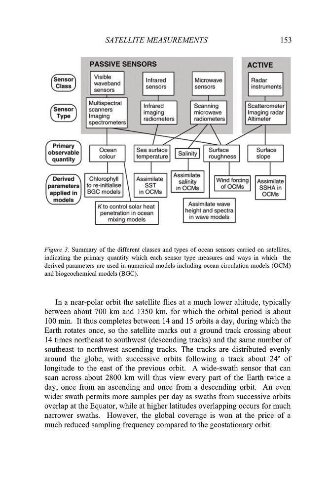
Figure 3. Summary of the different classes and types of ocean sensors carried on satellites,
indicating the primary quantity which each sensor type measures and ways in which the
derived parameters are used in numerical models including ocean circulation models (OCM)
and biogeochemical models (BGC).
In a near-polar orbit the satellite flies at a much lower altitude, typically
between about 700 km and 1350 km, for which the orbital period is about
100 min. It thus completes between 14 and 15 orbits a day, during which the
Earth rotates once, so the satellite marks out a ground track crossing about
14 times northeast to southwest (descending tracks) and the same number of
southeast to northwest ascending tracks. The tracks are distributed evenly
around the globe, with successive orbits following a track about 24º of
longitude to the east of the previous orbit. A wide-swath sensor that can
scan across about 2800 km will thus view every part of the Earth twice a
day, once from an ascending and once from a descending orbit. An even
wider swath permits more samples per day as swaths from successive orbits
overlap at the Equator, while at higher latitudes overlapping occurs for much
narrower swaths. However, the global coverage is won at the price of a
much reduced sampling frequency compared to the geostationary orbit.
153
Figure 3. Summary of the different classes and types of ocean sensors carried on satellites,
indicating the primary quantity which each sensor type measures and ways in which the
derived parameters are used in numerical models including ocean circulation models (OCM)
and biogeochemical models (BGC).
In a near-polar orbit the satellite flies at a much lower altitude, typically
between about 700 km and 1350 km, for which the orbital period is about
100 min. It thus completes between 14 and 15 orbits a day, during which the
Earth rotates once, so the satellite marks out a ground track crossing about
14 times northeast to southwest (descending tracks) and the same number of
southeast to northwest ascending tracks. The tracks are distributed evenly
around the globe, with successive orbits following a track about 24º of
longitude to the east of the previous orbit. A wide-swath sensor that can
scan across about 2800 km will thus view every part of the Earth twice a
day, once from an ascending and once from a descending orbit. An even
wider swath permits more samples per day as swaths from successive orbits
overlap at the Equator, while at higher latitudes overlapping occurs for much
narrower swaths. However, the global coverage is won at the price of a
much reduced sampling frequency compared to the geostationary orbit.