

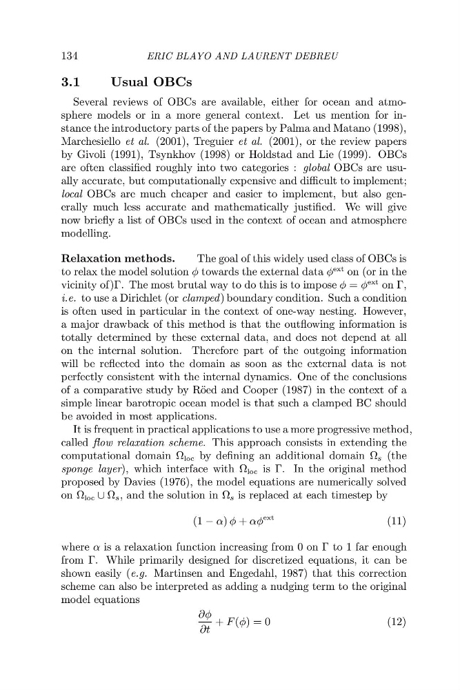
134
ERIC BLAYO AND LAURENT DEBREU
3.1
Usual OBCs
Several reviews of OBCs are available, either for ocean and atmosphere models or in a more general context. Let us mention for instance the introductory parts of the papers by Palma and Matano (1998),
Marchesiello et al. (2001), Treguier et al. (2001), or the review papers
by Givoli (1991), Tsynkhov (1998) or Holdstad and Lie (1999). OBCs
are often classified roughly into two categories : global OBCs are usually accurate, but computationally expensive and difficult to implement;
local OBCs are much cheaper and easier to implement, but also generally much less accurate and mathematically justified. We will give
now briefly a list of OBCs used in the context of ocean and atmosphere
modelling.
Relaxation methods.
The goal of this widely used class of OBCs is
to relax the model solution φ towards the external data φ
ext on (or in the
vicinity of)Γ. The most brutal way to do this is to impose φ = φ
ext on Γ,
i.e. to use a Dirichlet (or clamped ) boundary condition. Such a condition
is often used in particular in the context of one-way nesting. However,
a major drawback of this method is that the outflowing information is
totally determined by these external data, and does not depend at all
on the internal solution. Therefore part of the outgoing information
will be reflected into the domain as soon as the external data is not
perfectly consistent with the internal dynamics. One of the conclusions
of a comparative study by R¨ oed and Cooper (1987) in the context of a
simple linear barotropic ocean model is that such a clamped BC should
be avoided in most applications.
It is frequent in practical applications to use a more progressive method,
called flow relaxation scheme. This approach consists in extending the
computational domain Ω loc by defining an additional domain Ω s (the
sponge layer), which interface with Ω loc is Γ. In the original method
proposed by Davies (1976), the model equations are numerically solved
on Ω loc ∪ Ω s , and the solution in Ω s is replaced at each timestep by
(1 − α) φ + αφ
ext
(11)
where α is a relaxation function increasing from 0 on Γ to 1 far enough
from Γ. While primarily designed for discretized equations, it can be
shown easily (e.g. Martinsen and Engedahl, 1987) that this correction
scheme can also be interpreted as adding a nudging term to the original
model equations
∂φ
∂t
+ F (φ) = 0
(12)
ERIC BLAYO AND LAURENT DEBREU
3.1
Usual OBCs
Several reviews of OBCs are available, either for ocean and atmosphere models or in a more general context. Let us mention for instance the introductory parts of the papers by Palma and Matano (1998),
Marchesiello et al. (2001), Treguier et al. (2001), or the review papers
by Givoli (1991), Tsynkhov (1998) or Holdstad and Lie (1999). OBCs
are often classified roughly into two categories : global OBCs are usually accurate, but computationally expensive and difficult to implement;
local OBCs are much cheaper and easier to implement, but also generally much less accurate and mathematically justified. We will give
now briefly a list of OBCs used in the context of ocean and atmosphere
modelling.
Relaxation methods.
The goal of this widely used class of OBCs is
to relax the model solution φ towards the external data φ
ext on (or in the
vicinity of)Γ. The most brutal way to do this is to impose φ = φ
ext on Γ,
i.e. to use a Dirichlet (or clamped ) boundary condition. Such a condition
is often used in particular in the context of one-way nesting. However,
a major drawback of this method is that the outflowing information is
totally determined by these external data, and does not depend at all
on the internal solution. Therefore part of the outgoing information
will be reflected into the domain as soon as the external data is not
perfectly consistent with the internal dynamics. One of the conclusions
of a comparative study by R¨ oed and Cooper (1987) in the context of a
simple linear barotropic ocean model is that such a clamped BC should
be avoided in most applications.
It is frequent in practical applications to use a more progressive method,
called flow relaxation scheme. This approach consists in extending the
computational domain Ω loc by defining an additional domain Ω s (the
sponge layer), which interface with Ω loc is Γ. In the original method
proposed by Davies (1976), the model equations are numerically solved
on Ω loc ∪ Ω s , and the solution in Ω s is replaced at each timestep by
(1 − α) φ + αφ
ext
(11)
where α is a relaxation function increasing from 0 on Γ to 1 far enough
from Γ. While primarily designed for discretized equations, it can be
shown easily (e.g. Martinsen and Engedahl, 1987) that this correction
scheme can also be interpreted as adding a nudging term to the original
model equations
∂φ
∂t
+ F (φ) = 0
(12)