

NESTING OCEAN MODELS
133
0
0.1
0.2
0.3
0.4
0.5
0.6
0.7
0.8
0.9
1
0.1
0.15
0.2
0.25
0.3
0.35
0.4
0
0.1
0.2
0.3
0.4
0.5
0.6
0.7
0.8
0.9
1
−0.05
−0.04
−0.03
−0.02
−0.01
0
0.01
0.02
0.03
0.04
0.05
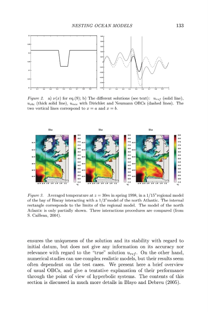
Figure 2. a) ν(x) for eq.(9); b) The different solutions (see text): u ref (solid line),
u obc (thick solid line), unes with Dirichlet and Neumann OBCs (dashed lines). The
two vertical lines correspond to x = a and x = b.
Figure 3. Averaged temperature at z = 30m in spring 1998, in a 1/15
◦ regional model
of the bay of Biscay interacting with a 1/3
◦ model of the north Atlantic. The internal
rectangle corresponds to the limits of the regional model. The model of the north
Atlantic is only partially shown. Three interactions procedures are compared (from
S. Cailleau, 2004).
ensures the uniqueness of the solution and its stability with regard to
initial datum, but does not give any information on its accuracy nor
relevance with regard to the “true” solution u ref . On the other hand,
numerical studies can use complex realistic models, but their results seem
often dependent on the test cases. We present here a brief overview
of usual OBCs, and give a tentative explanation of their performance
through the point of view of hyperbolic systems. The contents of this
section is discussed in much more details in Blayo and Debreu (2005).
133
0
0.1
0.2
0.3
0.4
0.5
0.6
0.7
0.8
0.9
1
0.1
0.15
0.2
0.25
0.3
0.35
0.4
0
0.1
0.2
0.3
0.4
0.5
0.6
0.7
0.8
0.9
1
−0.05
−0.04
−0.03
−0.02
−0.01
0
0.01
0.02
0.03
0.04
0.05
Figure 2. a) ν(x) for eq.(9); b) The different solutions (see text): u ref (solid line),
u obc (thick solid line), unes with Dirichlet and Neumann OBCs (dashed lines). The
two vertical lines correspond to x = a and x = b.
Figure 3. Averaged temperature at z = 30m in spring 1998, in a 1/15
◦ regional model
of the bay of Biscay interacting with a 1/3
◦ model of the north Atlantic. The internal
rectangle corresponds to the limits of the regional model. The model of the north
Atlantic is only partially shown. Three interactions procedures are compared (from
S. Cailleau, 2004).
ensures the uniqueness of the solution and its stability with regard to
initial datum, but does not give any information on its accuracy nor
relevance with regard to the “true” solution u ref . On the other hand,
numerical studies can use complex realistic models, but their results seem
often dependent on the test cases. We present here a brief overview
of usual OBCs, and give a tentative explanation of their performance
through the point of view of hyperbolic systems. The contents of this
section is discussed in much more details in Blayo and Debreu (2005).