

HYBRID VERTICAL COORDINATES
115
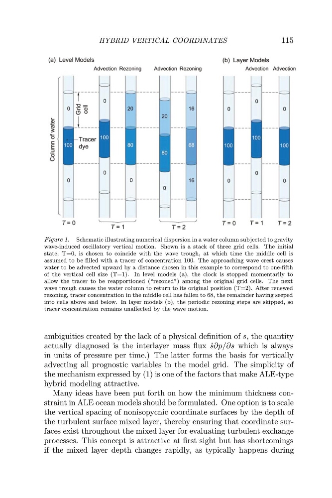
Figure 1. Schematic illustrating numerical dispersion in a water column subjected to gravity
wave-induced oscillatory vertical motion. Shown is a stack of three grid cells. The initial
state, T=0, is chosen to coincide with the wave trough, at which time the middle cell is
assumed to be filled with a tracer of concentration 100. The approaching wave crest causes
water to be advected upward by a distance chosen in this example to correspond to one-fifth
of the vertical cell size (T=1). In level models (a), the clock is stopped momentarily to
allow the tracer to be reapportioned (“rezoned”) among the original grid cells. The next
wave trough causes the water column to return to its original position (T=2). After renewed
rezoning, tracer concentration in the middle cell has fallen to 68, the remainder having seeped
into cells above and below. In layer models (b), the periodic rezoning steps are skipped, so
tracer concentration remains unaffected by the wave motion.
ambiguities created by the lack of a physical definition of s, the quantity
actually diagnosed is the interlayer mass flux ˙
s∂p/∂s which is always
in units of pressure per time.) The latter forms the basis for vertically
advecting all prognostic variables in the model grid. The simplicity of
the mechanism expressed by (1) is one of the factors that make ALE-type
hybrid modeling attractive.
Many ideas have been put forth on how the minimum thickness constraint in ALE ocean models should be formulated. One option is to scale
the vertical spacing of nonisopycnic coordinate surfaces by the depth of
the turbulent surface mixed layer, thereby ensuring that coordinate surfaces exist throughout the mixed layer for evaluating turbulent exchange
processes. This concept is attractive at first sight but has shortcomings
if the mixed layer depth changes rapidly, as typically happens during
115
Figure 1. Schematic illustrating numerical dispersion in a water column subjected to gravity
wave-induced oscillatory vertical motion. Shown is a stack of three grid cells. The initial
state, T=0, is chosen to coincide with the wave trough, at which time the middle cell is
assumed to be filled with a tracer of concentration 100. The approaching wave crest causes
water to be advected upward by a distance chosen in this example to correspond to one-fifth
of the vertical cell size (T=1). In level models (a), the clock is stopped momentarily to
allow the tracer to be reapportioned (“rezoned”) among the original grid cells. The next
wave trough causes the water column to return to its original position (T=2). After renewed
rezoning, tracer concentration in the middle cell has fallen to 68, the remainder having seeped
into cells above and below. In layer models (b), the periodic rezoning steps are skipped, so
tracer concentration remains unaffected by the wave motion.
ambiguities created by the lack of a physical definition of s, the quantity
actually diagnosed is the interlayer mass flux ˙
s∂p/∂s which is always
in units of pressure per time.) The latter forms the basis for vertically
advecting all prognostic variables in the model grid. The simplicity of
the mechanism expressed by (1) is one of the factors that make ALE-type
hybrid modeling attractive.
Many ideas have been put forth on how the minimum thickness constraint in ALE ocean models should be formulated. One option is to scale
the vertical spacing of nonisopycnic coordinate surfaces by the depth of
the turbulent surface mixed layer, thereby ensuring that coordinate surfaces exist throughout the mixed layer for evaluating turbulent exchange
processes. This concept is attractive at first sight but has shortcomings
if the mixed layer depth changes rapidly, as typically happens during