

114
RAINER BLECK
In summary, grid generation in HYCOM is a two-step process. In step
1, interfaces are set in motion to restore the target density in individual
layers. In step 2, this migration is checked for compatibility with an
imposed minimum thickness constraint. Step 2 overrides step 1.
The details of the minimum thickness constraint are essentially the
model designer’s choice. For example, during HYCOM development the
decision was made to impose nonzero-thickness constraints only at the
surface but allow layers at the bottom to become massless. This is done
for a good reason. Steeply inclined coordinate layers, like those following the bathymetry, are prone to errors in the horizontal pressure force
calculation. In a layer containing no mass, such errors are dynamically
inconsequential.
Complications arising from the grid generator’s ad-hoc strategy for
vertical grid point placement are minimal. This can be demonstrated as
follows (Bleck, 1978). Recall that material vertical motion in hydrostatic
models is inferred from mass continuity — specifically, from the vertically
integrated horizontal mass flux divergence. The material vertical motion
so diagnosed is then decomposed into motion of the coordinate surface
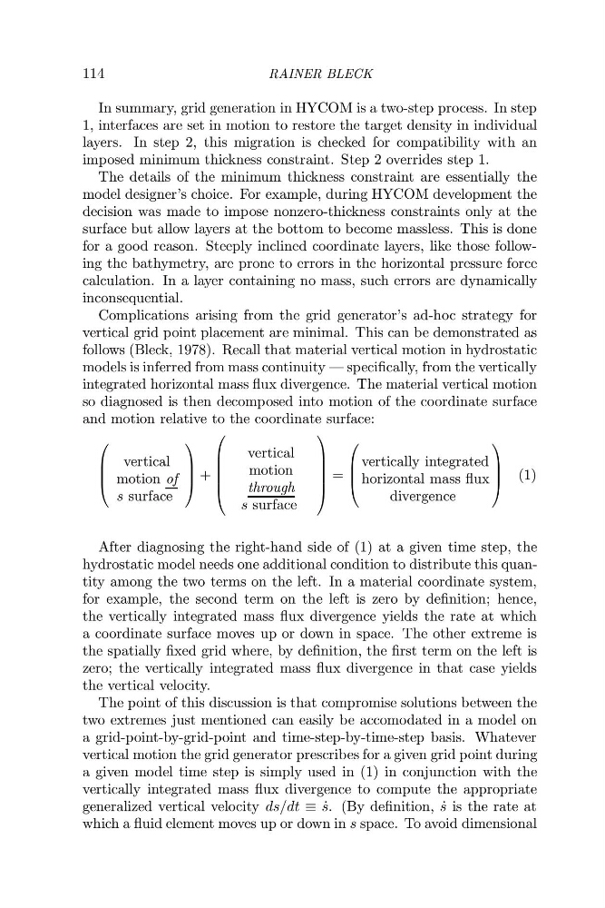
and motion relative to the coordinate surface:
⎛
⎜
⎜
⎝
vertical
motion of
s surface
⎞
⎟
⎟
⎠ +
⎛
⎜
⎜
⎜
⎜
⎝
vertical
motion
through
s surface
⎞
⎟
⎟
⎟
⎟
⎠
=
⎛
⎜
⎜
⎝
vertically integrated
horizontal mass flux
divergence
⎞
⎟
⎟
⎠ (1)
After diagnosing the right-hand side of (1) at a given time step, the
hydrostatic model needs one additional condition to distribute this quantity among the two terms on the left. In a material coordinate system,
for example, the second term on the left is zero by definition; hence,
the vertically integrated mass flux divergence yields the rate at which
a coordinate surface moves up or down in space. The other extreme is
the spatially fixed grid where, by definition, the first term on the left is
zero; the vertically integrated mass flux divergence in that case yields
the vertical velocity.
The point of this discussion is that compromise solutions between the
two extremes just mentioned can easily be accomodated in a model on
a grid-point-by-grid-point and time-step-by-time-step basis. Whatever
vertical motion the grid generator prescribes for a given grid point during
a given model time step is simply used in (1) in conjunction with the
vertically integrated mass flux divergence to compute the appropriate
generalized vertical velocity ds/dt ≡ ˙
s. (By definition, ˙
s is the rate at
which a fluid element moves up or down in s space. To avoid dimensional
RAINER BLECK
In summary, grid generation in HYCOM is a two-step process. In step
1, interfaces are set in motion to restore the target density in individual
layers. In step 2, this migration is checked for compatibility with an
imposed minimum thickness constraint. Step 2 overrides step 1.
The details of the minimum thickness constraint are essentially the
model designer’s choice. For example, during HYCOM development the
decision was made to impose nonzero-thickness constraints only at the
surface but allow layers at the bottom to become massless. This is done
for a good reason. Steeply inclined coordinate layers, like those following the bathymetry, are prone to errors in the horizontal pressure force
calculation. In a layer containing no mass, such errors are dynamically
inconsequential.
Complications arising from the grid generator’s ad-hoc strategy for
vertical grid point placement are minimal. This can be demonstrated as
follows (Bleck, 1978). Recall that material vertical motion in hydrostatic
models is inferred from mass continuity — specifically, from the vertically
integrated horizontal mass flux divergence. The material vertical motion
so diagnosed is then decomposed into motion of the coordinate surface
and motion relative to the coordinate surface:
⎛
⎜
⎜
⎝
vertical
motion of
s surface
⎞
⎟
⎟
⎠ +
⎛
⎜
⎜
⎜
⎜
⎝
vertical
motion
through
s surface
⎞
⎟
⎟
⎟
⎟
⎠
=
⎛
⎜
⎜
⎝
vertically integrated
horizontal mass flux
divergence
⎞
⎟
⎟
⎠ (1)
After diagnosing the right-hand side of (1) at a given time step, the
hydrostatic model needs one additional condition to distribute this quantity among the two terms on the left. In a material coordinate system,
for example, the second term on the left is zero by definition; hence,
the vertically integrated mass flux divergence yields the rate at which
a coordinate surface moves up or down in space. The other extreme is
the spatially fixed grid where, by definition, the first term on the left is
zero; the vertically integrated mass flux divergence in that case yields
the vertical velocity.
The point of this discussion is that compromise solutions between the
two extremes just mentioned can easily be accomodated in a model on
a grid-point-by-grid-point and time-step-by-time-step basis. Whatever
vertical motion the grid generator prescribes for a given grid point during
a given model time step is simply used in (1) in conjunction with the
vertically integrated mass flux divergence to compute the appropriate
generalized vertical velocity ds/dt ≡ ˙
s. (By definition, ˙
s is the rate at
which a fluid element moves up or down in s space. To avoid dimensional