

3.22 Exercise 13: Stratified Flows on a Slope
81
is only useful in situations in which the plume is void of entrainment of ambient
fluid. Laboratory experiments suggest that, owing to entrainment, the velocity of
the plume head is almost independent of the slope angle (Britter and Linden, 1980).
Influence of the Coriolis force, not considered here, can also substantially modify
the dynamics. This will take place on time scales exceeding the inertial period.
The above equations are very similar to those used in previous exercises, apart
from an additional term in the bottom-parallel component of the momentum equation and a slight modification of the hydrostatic part of pressure when adjusted
parallel to the z r direction. Hence, only minor code modifications are required for
simulations of density-driven flows on a sloping sea floor.
3.22 Exercise 13: Stratified Flows on a Slope
3.22.1 Aim
The aim of this exercise is to employ a tilted Cartesian coordinate system to simulate
the dynamics and instability of a stratified flow on a sea floor of uniform slope.
3.22.2 Task Description
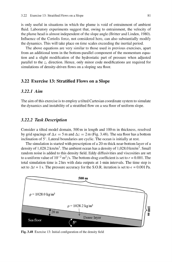
Consider a tilted model domain, 500 m in length and 100 m in thickness, resolved
by grid spacings of Δx = 5 m and Δz = 2 m (Fig. 3.48). The sea floor has a bottom
inclination of 5
◦ . Lateral boundaries are cyclic. The ocean is initially at rest.
The simulation is started with prescription of a 20-m thick near-bottom layer of a
density of 1,028.2 km/m
3 . The ambient ocean has a density of 1,028.0 km/m
3 . Small
random noise is added to this density field. Eddy diffusivities and viscosities are set
to a uniform value of 10
−2 m
2
/s. The bottom-drag coefficient is set to r = 0.001. The
total simulation time is 2 hrs with data outputs at 1-min intervals. The time step is
set to Δt = 1 s. The pressure accuracy for the S.O.R. iteration is set to = 0.001 Pa.
Fig. 3.48 Exercise 13: Initial configuration of the density field
81
is only useful in situations in which the plume is void of entrainment of ambient
fluid. Laboratory experiments suggest that, owing to entrainment, the velocity of
the plume head is almost independent of the slope angle (Britter and Linden, 1980).
Influence of the Coriolis force, not considered here, can also substantially modify
the dynamics. This will take place on time scales exceeding the inertial period.
The above equations are very similar to those used in previous exercises, apart
from an additional term in the bottom-parallel component of the momentum equation and a slight modification of the hydrostatic part of pressure when adjusted
parallel to the z r direction. Hence, only minor code modifications are required for
simulations of density-driven flows on a sloping sea floor.
3.22 Exercise 13: Stratified Flows on a Slope
3.22.1 Aim
The aim of this exercise is to employ a tilted Cartesian coordinate system to simulate
the dynamics and instability of a stratified flow on a sea floor of uniform slope.
3.22.2 Task Description
Consider a tilted model domain, 500 m in length and 100 m in thickness, resolved
by grid spacings of Δx = 5 m and Δz = 2 m (Fig. 3.48). The sea floor has a bottom
inclination of 5
◦ . Lateral boundaries are cyclic. The ocean is initially at rest.
The simulation is started with prescription of a 20-m thick near-bottom layer of a
density of 1,028.2 km/m
3 . The ambient ocean has a density of 1,028.0 km/m
3 . Small
random noise is added to this density field. Eddy diffusivities and viscosities are set
to a uniform value of 10
−2 m
2
/s. The bottom-drag coefficient is set to r = 0.001. The
total simulation time is 2 hrs with data outputs at 1-min intervals. The time step is
set to Δt = 1 s. The pressure accuracy for the S.O.R. iteration is set to = 0.001 Pa.
Fig. 3.48 Exercise 13: Initial configuration of the density field