

3.15 Exercise 8: Free Convection
61
3.15.2 Task Description
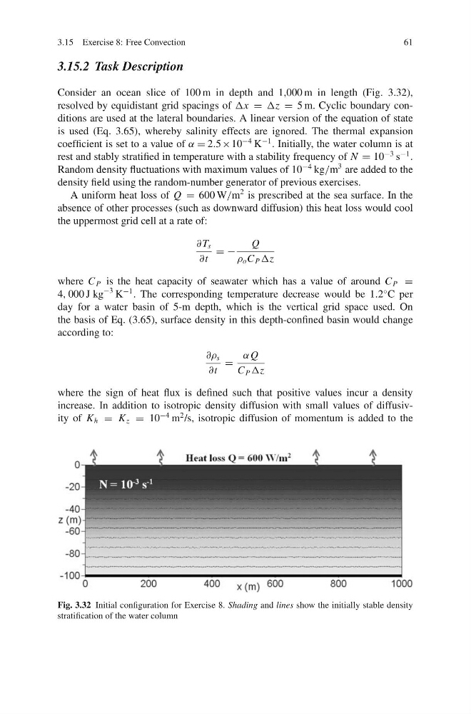
Consider an ocean slice of 100 m in depth and 1,000 m in length (Fig. 3.32),
resolved by equidistant grid spacings of Δx = Δz = 5 m. Cyclic boundary conditions are used at the lateral boundaries. A linear version of the equation of state
is used (Eq. 3.65), whereby salinity effects are ignored. The thermal expansion
coefficient is set to a value of α = 2.5×10
−4 K
−1 . Initially, the water column is at
rest and stably stratified in temperature with a stability frequency of N = 10
−3 s
−1 .
Random density fluctuations with maximum values of 10
−4 kg/m
3 are added to the
density field using the random-number generator of previous exercises.
A uniform heat loss of Q = 600 W/m
2 is prescribed at the sea surface. In the
absence of other processes (such as downward diffusion) this heat loss would cool
the uppermost grid cell at a rate of:
∂ T s
∂t
= −
Q
ρ o C P Δz
where C P is the heat capacity of seawater which has a value of around C P =
4, 000 J kg
−3 K
−1 . The corresponding temperature decrease would be 1.2
◦ C per
day for a water basin of 5-m depth, which is the vertical grid space used. On
the basis of Eq. (3.65), surface density in this depth-confined basin would change
according to:
∂ρ s
∂t
=
α Q
C P Δz
where the sign of heat flux is defined such that positive values incur a density
increase. In addition to isotropic density diffusion with small values of diffusivity of K h = K z = 10
−4 m
2 /s, isotropic diffusion of momentum is added to the
Fig. 3.32 Initial configuration for Exercise 8. Shading and lines show the initially stable density
stratification of the water column
61
3.15.2 Task Description
Consider an ocean slice of 100 m in depth and 1,000 m in length (Fig. 3.32),
resolved by equidistant grid spacings of Δx = Δz = 5 m. Cyclic boundary conditions are used at the lateral boundaries. A linear version of the equation of state
is used (Eq. 3.65), whereby salinity effects are ignored. The thermal expansion
coefficient is set to a value of α = 2.5×10
−4 K
−1 . Initially, the water column is at
rest and stably stratified in temperature with a stability frequency of N = 10
−3 s
−1 .
Random density fluctuations with maximum values of 10
−4 kg/m
3 are added to the
density field using the random-number generator of previous exercises.
A uniform heat loss of Q = 600 W/m
2 is prescribed at the sea surface. In the
absence of other processes (such as downward diffusion) this heat loss would cool
the uppermost grid cell at a rate of:
∂ T s
∂t
= −
Q
ρ o C P Δz
where C P is the heat capacity of seawater which has a value of around C P =
4, 000 J kg
−3 K
−1 . The corresponding temperature decrease would be 1.2
◦ C per
day for a water basin of 5-m depth, which is the vertical grid space used. On
the basis of Eq. (3.65), surface density in this depth-confined basin would change
according to:
∂ρ s
∂t
=
α Q
C P Δz
where the sign of heat flux is defined such that positive values incur a density
increase. In addition to isotropic density diffusion with small values of diffusivity of K h = K z = 10
−4 m
2 /s, isotropic diffusion of momentum is added to the
Fig. 3.32 Initial configuration for Exercise 8. Shading and lines show the initially stable density
stratification of the water column