

40
3 Basics of Nonhydrostatic Modelling
With inclusion of the nonlinear terms (required for subsequent exercises), the
first-guess value of velocity is now calculated from:
u
∗
i,k = u
n
i,k − ΔtAdv(u) −
Δt
ρ o Δx
( p
n
i,k+1 − p
n
i,k + q
n
i,k+1 − q
n
i,k )
(3.45)
w
∗
i,k = w
n
i,k − ΔtAdv(w) −
Δt
ρ o Δz
( p
n
i−1,k − p
n
i,k + q
n
i−1,k − q
n
i,k ) (3.46)
where Adv(u) and Adv(w) represent the nonlinear terms.
3.7 Exercise 4: Density-Driven Flows
3.7.1 Aim
The aim of this exercise is to apply the vertical ocean-slice model in a study of
bottom-arrested density-driven flows over variable bottom topography.
3.7.2 Task Description
Consider a closed channel, 500 m long and 100 m deep, resolved by grid spacings
of Δx = 5 m and Δz = 2 m. This configuration is the same as in Exercise 3. The
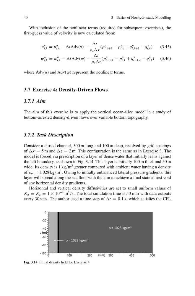
model is forced via prescription of a layer of dense water that initially leans against
the left boundary, as shown in Fig. 3.14. This layer is initially 100 m thick and 50 m
wide. Its density is 1 kg/m
3 greater compared with ambient water having a density
of ρ o = 1,028 kg/m
3 . Owing to initially unbalanced lateral pressure gradients, this
layer will spread along the sea floor with the aim to achieve a final state at rest void
of any horizontal density gradients.
Horizontal and vertical density diffusivities are set to small uniform values of
K h = K z = 1 × 10
−4 m
2
/s. The total simulation time is 50 min with data outputs
every 30 secs. The author used a time step of Δt = 0.1 s, which satisfies the CFL
Fig. 3.14 Initial density field for Exercise 4
3 Basics of Nonhydrostatic Modelling
With inclusion of the nonlinear terms (required for subsequent exercises), the
first-guess value of velocity is now calculated from:
u
∗
i,k = u
n
i,k − ΔtAdv(u) −
Δt
ρ o Δx
( p
n
i,k+1 − p
n
i,k + q
n
i,k+1 − q
n
i,k )
(3.45)
w
∗
i,k = w
n
i,k − ΔtAdv(w) −
Δt
ρ o Δz
( p
n
i−1,k − p
n
i,k + q
n
i−1,k − q
n
i,k ) (3.46)
where Adv(u) and Adv(w) represent the nonlinear terms.
3.7 Exercise 4: Density-Driven Flows
3.7.1 Aim
The aim of this exercise is to apply the vertical ocean-slice model in a study of
bottom-arrested density-driven flows over variable bottom topography.
3.7.2 Task Description
Consider a closed channel, 500 m long and 100 m deep, resolved by grid spacings
of Δx = 5 m and Δz = 2 m. This configuration is the same as in Exercise 3. The
model is forced via prescription of a layer of dense water that initially leans against
the left boundary, as shown in Fig. 3.14. This layer is initially 100 m thick and 50 m
wide. Its density is 1 kg/m
3 greater compared with ambient water having a density
of ρ o = 1,028 kg/m
3 . Owing to initially unbalanced lateral pressure gradients, this
layer will spread along the sea floor with the aim to achieve a final state at rest void
of any horizontal density gradients.
Horizontal and vertical density diffusivities are set to small uniform values of
K h = K z = 1 × 10
−4 m
2
/s. The total simulation time is 50 min with data outputs
every 30 secs. The author used a time step of Δt = 0.1 s, which satisfies the CFL
Fig. 3.14 Initial density field for Exercise 4