

3.6 Inclusion of Variable Density
39
where the interpolated values of eddy diffusivity are given by:
K
e
h = 0.5
K h,i,k + K h,i,k+1
and K
w
h = 0.5
K h,i,k + K h,i,k−1
K
+
z = 0.5
K z,i,k + K z,i−1,k
and K
−
z = 0.5
K z,i,k + K z,i+1,k
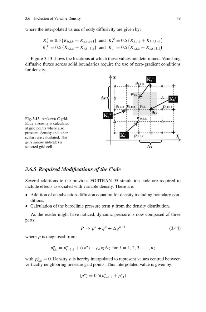
Figure 3.13 shows the locations at which these values are determined. Vanishing
diffusive fluxes across solid boundaries require the use of zero-gradient conditions
for density.
Fig. 3.13 Arakawa-C grid.
Eddy viscosity is calculated
at grid points where also
pressure, density and other
scalars are calculated. The
gray square indicates a
selected grid cell
3.6.5 Required Modifications of the Code
Several additions to the previous FORTRAN 95 simulation code are required to
include effects associated with variable density. These are:
• Addition of an advection-diffusion equation for density including boundary conditions,
• Calculation of the baroclinic pressure term p from the density distribution.
As the reader might have noticed, dynamic pressure is now composed of three
parts:
P ⇒ p
n
+ q
n
+ Δq
n+1
(3.44)
where p is diagnosed from:
p
n
i,k = p
n
i−1,k + (ρ
n
− ρ o )gΔz for i = 1, 2, 3, · · · , nz
with p
n
0,k = 0. Density ρ is hereby interpolated to represent values centred between
vertically neighboring pressure grid points. This interpolated value is given by:
ρ
n
= 0.5(ρ
n
i−1,k + ρ
n
i,k )
39
where the interpolated values of eddy diffusivity are given by:
K
e
h = 0.5
K h,i,k + K h,i,k+1
and K
w
h = 0.5
K h,i,k + K h,i,k−1
K
+
z = 0.5
K z,i,k + K z,i−1,k
and K
−
z = 0.5
K z,i,k + K z,i+1,k
Figure 3.13 shows the locations at which these values are determined. Vanishing
diffusive fluxes across solid boundaries require the use of zero-gradient conditions
for density.
Fig. 3.13 Arakawa-C grid.
Eddy viscosity is calculated
at grid points where also
pressure, density and other
scalars are calculated. The
gray square indicates a
selected grid cell
3.6.5 Required Modifications of the Code
Several additions to the previous FORTRAN 95 simulation code are required to
include effects associated with variable density. These are:
• Addition of an advection-diffusion equation for density including boundary conditions,
• Calculation of the baroclinic pressure term p from the density distribution.
As the reader might have noticed, dynamic pressure is now composed of three
parts:
P ⇒ p
n
+ q
n
+ Δq
n+1
(3.44)
where p is diagnosed from:
p
n
i,k = p
n
i−1,k + (ρ
n
− ρ o )gΔz for i = 1, 2, 3, · · · , nz
with p
n
0,k = 0. Density ρ is hereby interpolated to represent values centred between
vertically neighboring pressure grid points. This interpolated value is given by:
ρ
n
= 0.5(ρ
n
i−1,k + ρ
n
i,k )