

3.2 2D Vertical-Slice Modelling
23
Fig. 3.2 The two-dimensional vertical ocean slice
The continuity equation (Eq. 1.2) can be written as:
∂u
∂ x
+
∂w
∂z
= 0
(3.2)
3.2.2 The Arakawa C-Grid
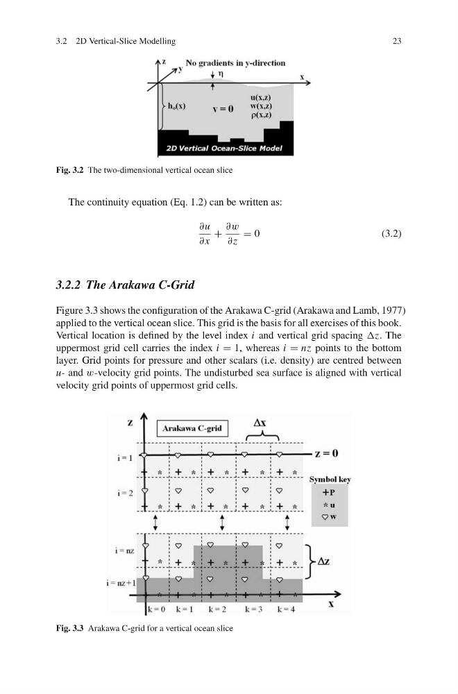
Figure 3.3 shows the configuration of the Arakawa C-grid (Arakawa and Lamb, 1977)
applied to the vertical ocean slice. This grid is the basis for all exercises of this book.
Vertical location is defined by the level index i and vertical grid spacing Δz. The
uppermost grid cell carries the index i = 1, whereas i = nz points to the bottom
layer. Grid points for pressure and other scalars (i.e. density) are centred between
u- and w-velocity grid points. The undisturbed sea surface is aligned with vertical
velocity grid points of uppermost grid cells.
Fig. 3.3 Arakawa C-grid for a vertical ocean slice
23
Fig. 3.2 The two-dimensional vertical ocean slice
The continuity equation (Eq. 1.2) can be written as:
∂u
∂ x
+
∂w
∂z
= 0
(3.2)
3.2.2 The Arakawa C-Grid
Figure 3.3 shows the configuration of the Arakawa C-grid (Arakawa and Lamb, 1977)
applied to the vertical ocean slice. This grid is the basis for all exercises of this book.
Vertical location is defined by the level index i and vertical grid spacing Δz. The
uppermost grid cell carries the index i = 1, whereas i = nz points to the bottom
layer. Grid points for pressure and other scalars (i.e. density) are centred between
u- and w-velocity grid points. The undisturbed sea surface is aligned with vertical
velocity grid points of uppermost grid cells.
Fig. 3.3 Arakawa C-grid for a vertical ocean slice