

156
5 3D Level Modelling
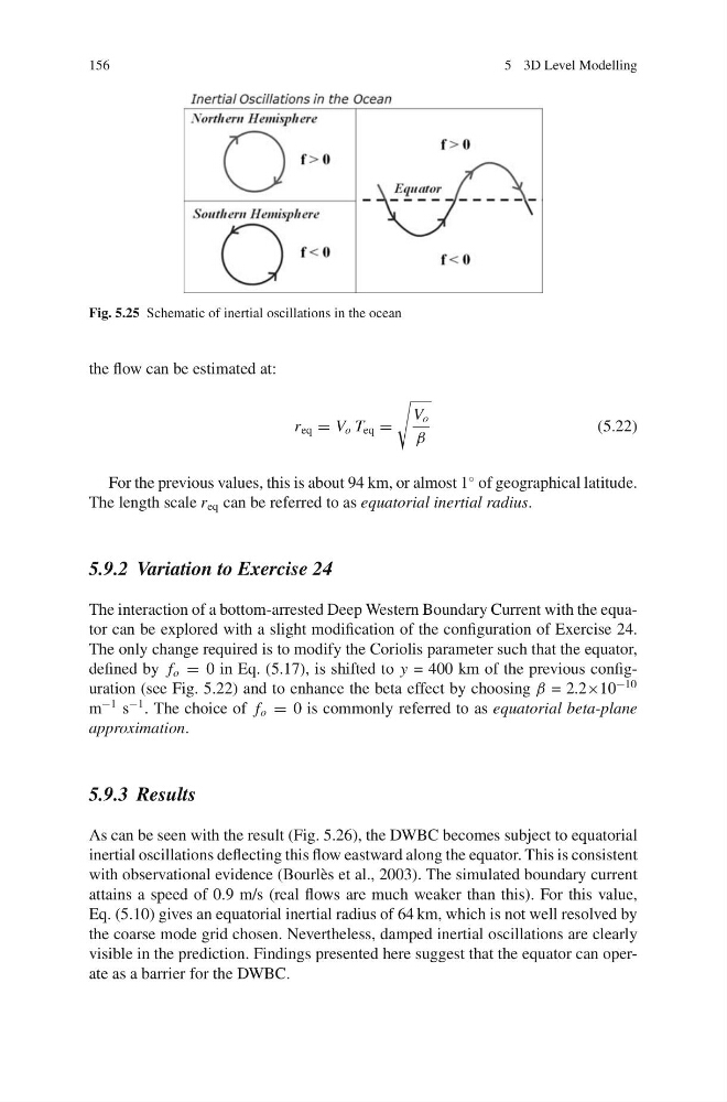
Fig. 5.25 Schematic of inertial oscillations in the ocean
the flow can be estimated at:
r eq = V o T eq =
V o
β
(5.22)
For the previous values, this is about 94 km, or almost 1
◦ of geographical latitude.
The length scale r eq can be referred to as equatorial inertial radius.
5.9.2 Variation to Exercise 24
The interaction of a bottom-arrested Deep Western Boundary Current with the equator can be explored with a slight modification of the configuration of Exercise 24.
The only change required is to modify the Coriolis parameter such that the equator,
defined by f o = 0 in Eq. (5.17), is shifted to y = 400 km of the previous configuration (see Fig. 5.22) and to enhance the beta effect by choosing β = 2.2×10
−10
m
−1 s
−1 . The choice of f o = 0 is commonly referred to as equatorial beta-plane
approximation.
5.9.3 Results
As can be seen with the result (Fig. 5.26), the DWBC becomes subject to equatorial
inertial oscillations deflecting this flow eastward along the equator. This is consistent
with observational evidence (Bourl` es et al., 2003). The simulated boundary current
attains a speed of 0.9 m/s (real flows are much weaker than this). For this value,
Eq. (5.10) gives an equatorial inertial radius of 64 km, which is not well resolved by
the coarse mode grid chosen. Nevertheless, damped inertial oscillations are clearly
visible in the prediction. Findings presented here suggest that the equator can operate as a barrier for the DWBC.
5 3D Level Modelling
Fig. 5.25 Schematic of inertial oscillations in the ocean
the flow can be estimated at:
r eq = V o T eq =
V o
β
(5.22)
For the previous values, this is about 94 km, or almost 1
◦ of geographical latitude.
The length scale r eq can be referred to as equatorial inertial radius.
5.9.2 Variation to Exercise 24
The interaction of a bottom-arrested Deep Western Boundary Current with the equator can be explored with a slight modification of the configuration of Exercise 24.
The only change required is to modify the Coriolis parameter such that the equator,
defined by f o = 0 in Eq. (5.17), is shifted to y = 400 km of the previous configuration (see Fig. 5.22) and to enhance the beta effect by choosing β = 2.2×10
−10
m
−1 s
−1 . The choice of f o = 0 is commonly referred to as equatorial beta-plane
approximation.
5.9.3 Results
As can be seen with the result (Fig. 5.26), the DWBC becomes subject to equatorial
inertial oscillations deflecting this flow eastward along the equator. This is consistent
with observational evidence (Bourl` es et al., 2003). The simulated boundary current
attains a speed of 0.9 m/s (real flows are much weaker than this). For this value,
Eq. (5.10) gives an equatorial inertial radius of 64 km, which is not well resolved by
the coarse mode grid chosen. Nevertheless, damped inertial oscillations are clearly
visible in the prediction. Findings presented here suggest that the equator can operate as a barrier for the DWBC.