

5.8 Exercise 24: The Abyssal Circulation
149
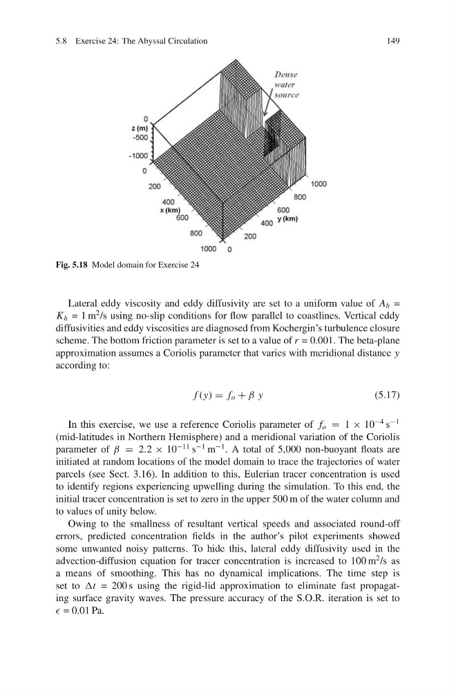
Fig. 5.18 Model domain for Exercise 24
Lateral eddy viscosity and eddy diffusivity are set to a uniform value of A h =
K h = 1 m
2 /s using no-slip conditions for flow parallel to coastlines. Vertical eddy
diffusivities and eddy viscosities are diagnosed from Kochergin’s turbulence closure
scheme. The bottom friction parameter is set to a value of r = 0.001. The beta-plane
approximation assumes a Coriolis parameter that varies with meridional distance y
according to:
f (y) = f o + β y
(5.17)
In this exercise, we use a reference Coriolis parameter of f o = 1 × 10
−4 s
−1
(mid-latitudes in Northern Hemisphere) and a meridional variation of the Coriolis
parameter of β = 2.2 × 10
−11 s
−1 m
−1 . A total of 5,000 non-buoyant floats are
initiated at random locations of the model domain to trace the trajectories of water
parcels (see Sect. 3.16). In addition to this, Eulerian tracer concentration is used
to identify regions experiencing upwelling during the simulation. To this end, the
initial tracer concentration is set to zero in the upper 500 m of the water column and
to values of unity below.
Owing to the smallness of resultant vertical speeds and associated round-off
errors, predicted concentration fields in the author’s pilot experiments showed
some unwanted noisy patterns. To hide this, lateral eddy diffusivity used in the
advection-diffusion equation for tracer concentration is increased to 100 m
2 /s as
a means of smoothing. This has no dynamical implications. The time step is
set to Δt = 200 s using the rigid-lid approximation to eliminate fast propagating surface gravity waves. The pressure accuracy of the S.O.R. iteration is set to
= 0.01 Pa.
149
Fig. 5.18 Model domain for Exercise 24
Lateral eddy viscosity and eddy diffusivity are set to a uniform value of A h =
K h = 1 m
2 /s using no-slip conditions for flow parallel to coastlines. Vertical eddy
diffusivities and eddy viscosities are diagnosed from Kochergin’s turbulence closure
scheme. The bottom friction parameter is set to a value of r = 0.001. The beta-plane
approximation assumes a Coriolis parameter that varies with meridional distance y
according to:
f (y) = f o + β y
(5.17)
In this exercise, we use a reference Coriolis parameter of f o = 1 × 10
−4 s
−1
(mid-latitudes in Northern Hemisphere) and a meridional variation of the Coriolis
parameter of β = 2.2 × 10
−11 s
−1 m
−1 . A total of 5,000 non-buoyant floats are
initiated at random locations of the model domain to trace the trajectories of water
parcels (see Sect. 3.16). In addition to this, Eulerian tracer concentration is used
to identify regions experiencing upwelling during the simulation. To this end, the
initial tracer concentration is set to zero in the upper 500 m of the water column and
to values of unity below.
Owing to the smallness of resultant vertical speeds and associated round-off
errors, predicted concentration fields in the author’s pilot experiments showed
some unwanted noisy patterns. To hide this, lateral eddy diffusivity used in the
advection-diffusion equation for tracer concentration is increased to 100 m
2 /s as
a means of smoothing. This has no dynamical implications. The time step is
set to Δt = 200 s using the rigid-lid approximation to eliminate fast propagating surface gravity waves. The pressure accuracy of the S.O.R. iteration is set to
= 0.01 Pa.