

148
5 3D Level Modelling
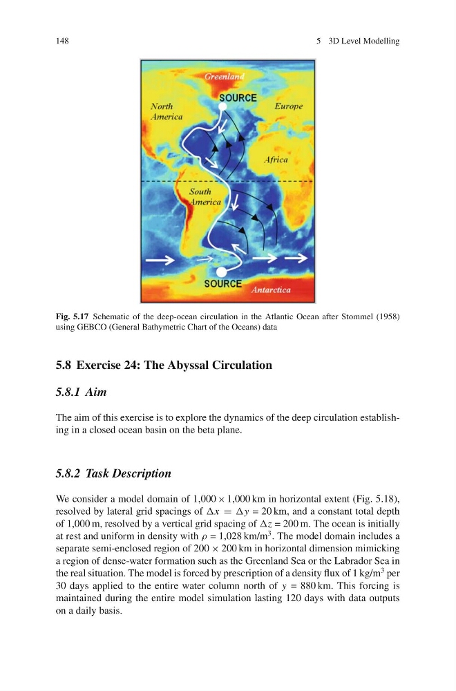
Fig. 5.17 Schematic of the deep-ocean circulation in the Atlantic Ocean after Stommel (1958)
using GEBCO (General Bathymetric Chart of the Oceans) data
5.8 Exercise 24: The Abyssal Circulation
5.8.1 Aim
The aim of this exercise is to explore the dynamics of the deep circulation establishing in a closed ocean basin on the beta plane.
5.8.2 Task Description
We consider a model domain of 1,000 × 1,000 km in horizontal extent (Fig. 5.18),
resolved by lateral grid spacings of Δx = Δy = 20 km, and a constant total depth
of 1,000 m, resolved by a vertical grid spacing of Δz = 200 m. The ocean is initially
at rest and uniform in density with ρ = 1,028 km/m
3 . The model domain includes a
separate semi-enclosed region of 200 × 200 km in horizontal dimension mimicking
a region of dense-water formation such as the Greenland Sea or the Labrador Sea in
the real situation. The model is forced by prescription of a density flux of 1 kg/m
3 per
30 days applied to the entire water column north of y = 880 km. This forcing is
maintained during the entire model simulation lasting 120 days with data outputs
on a daily basis.
5 3D Level Modelling
Fig. 5.17 Schematic of the deep-ocean circulation in the Atlantic Ocean after Stommel (1958)
using GEBCO (General Bathymetric Chart of the Oceans) data
5.8 Exercise 24: The Abyssal Circulation
5.8.1 Aim
The aim of this exercise is to explore the dynamics of the deep circulation establishing in a closed ocean basin on the beta plane.
5.8.2 Task Description
We consider a model domain of 1,000 × 1,000 km in horizontal extent (Fig. 5.18),
resolved by lateral grid spacings of Δx = Δy = 20 km, and a constant total depth
of 1,000 m, resolved by a vertical grid spacing of Δz = 200 m. The ocean is initially
at rest and uniform in density with ρ = 1,028 km/m
3 . The model domain includes a
separate semi-enclosed region of 200 × 200 km in horizontal dimension mimicking
a region of dense-water formation such as the Greenland Sea or the Labrador Sea in
the real situation. The model is forced by prescription of a density flux of 1 kg/m
3 per
30 days applied to the entire water column north of y = 880 km. This forcing is
maintained during the entire model simulation lasting 120 days with data outputs
on a daily basis.