

5.6 Exercise 23: Coastal Upwelling in 3D
145
5.6.4 Additional Exercise for the Reader
Repeat this exercise with an overall onshore (northward) wind stress. Does the east
facing coast of the bay support coastal upwelling?
5.6.5 Time-Splitting Methods
The reader will have noticed by now that three-dimensional model simulation are
fairly slow and take a long time to complete. The reason of this time-step compliance with the CFL criterion for fast propagating surface gravity waves (Eq. 5.15).
Enabling the rigid-lid condition (see Sect. 3.7) seems a solution, but this could lead
to a bias in the dynamics predicted. Another method is to use different numerical
time steps in different parts of the model code, a method called time splitting. To this
end, small time steps only need to be applied within the S.O.R. iteration involving
the surface pressure field, whereas all other parts such as advective and diffusive
changes can employ a much larger time step. Note that the latter still needs to satisfy
the stability criterion Eq. (5.14).
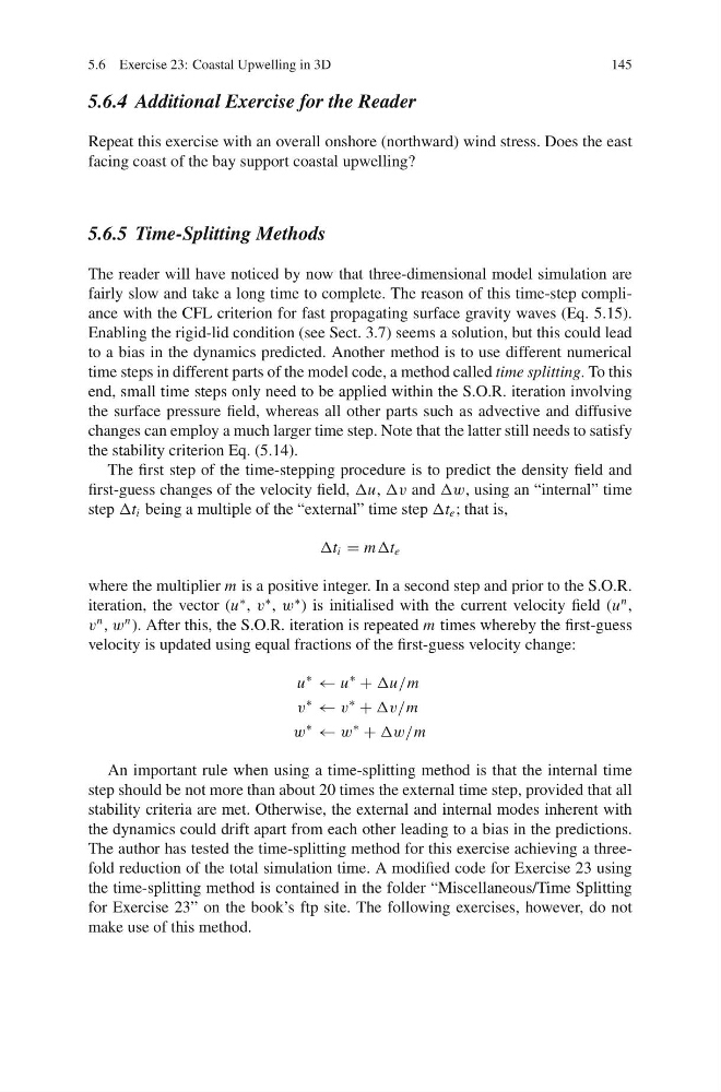
The first step of the time-stepping procedure is to predict the density field and
first-guess changes of the velocity field, Δu, Δv and Δw, using an “internal” time
step Δt i being a multiple of the “external” time step Δt e ; that is,
Δt i = mΔt e
where the multiplier m is a positive integer. In a second step and prior to the S.O.R.
iteration, the vector (u
∗ , v
∗ , w
∗ ) is initialised with the current velocity field (u
n ,
v
n , w
n ). After this, the S.O.R. iteration is repeated m times whereby the first-guess
velocity is updated using equal fractions of the first-guess velocity change:
u
∗
← u
∗
+ Δu/m
v
∗
← v
∗
+ Δv/m
w
∗
← w
∗
+ Δw/m
An important rule when using a time-splitting method is that the internal time
step should be not more than about 20 times the external time step, provided that all
stability criteria are met. Otherwise, the external and internal modes inherent with
the dynamics could drift apart from each other leading to a bias in the predictions.
The author has tested the time-splitting method for this exercise achieving a threefold reduction of the total simulation time. A modified code for Exercise 23 using
the time-splitting method is contained in the folder “Miscellaneous/Time Splitting
for Exercise 23” on the book’s ftp site. The following exercises, however, do not
make use of this method.
145
5.6.4 Additional Exercise for the Reader
Repeat this exercise with an overall onshore (northward) wind stress. Does the east
facing coast of the bay support coastal upwelling?
5.6.5 Time-Splitting Methods
The reader will have noticed by now that three-dimensional model simulation are
fairly slow and take a long time to complete. The reason of this time-step compliance with the CFL criterion for fast propagating surface gravity waves (Eq. 5.15).
Enabling the rigid-lid condition (see Sect. 3.7) seems a solution, but this could lead
to a bias in the dynamics predicted. Another method is to use different numerical
time steps in different parts of the model code, a method called time splitting. To this
end, small time steps only need to be applied within the S.O.R. iteration involving
the surface pressure field, whereas all other parts such as advective and diffusive
changes can employ a much larger time step. Note that the latter still needs to satisfy
the stability criterion Eq. (5.14).
The first step of the time-stepping procedure is to predict the density field and
first-guess changes of the velocity field, Δu, Δv and Δw, using an “internal” time
step Δt i being a multiple of the “external” time step Δt e ; that is,
Δt i = mΔt e
where the multiplier m is a positive integer. In a second step and prior to the S.O.R.
iteration, the vector (u
∗ , v
∗ , w
∗ ) is initialised with the current velocity field (u
n ,
v
n , w
n ). After this, the S.O.R. iteration is repeated m times whereby the first-guess
velocity is updated using equal fractions of the first-guess velocity change:
u
∗
← u
∗
+ Δu/m
v
∗
← v
∗
+ Δv/m
w
∗
← w
∗
+ Δw/m
An important rule when using a time-splitting method is that the internal time
step should be not more than about 20 times the external time step, provided that all
stability criteria are met. Otherwise, the external and internal modes inherent with
the dynamics could drift apart from each other leading to a bias in the predictions.
The author has tested the time-splitting method for this exercise achieving a threefold reduction of the total simulation time. A modified code for Exercise 23 using
the time-splitting method is contained in the folder “Miscellaneous/Time Splitting
for Exercise 23” on the book’s ftp site. The following exercises, however, do not
make use of this method.