

4.6 Exercise 19: Ekman Pumping
123
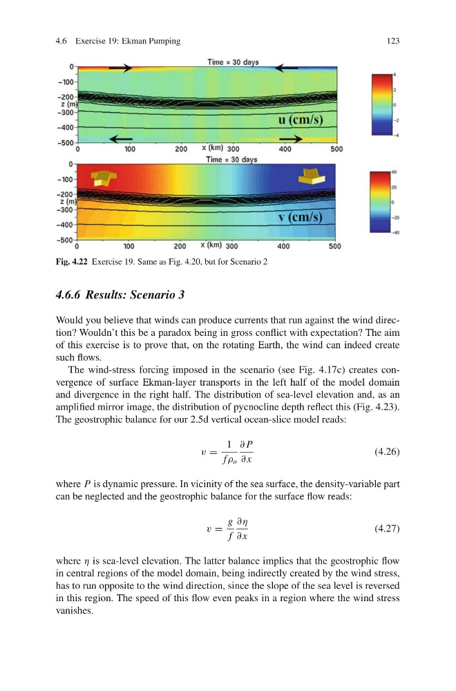
Fig. 4.22 Exercise 19. Same as Fig. 4.20, but for Scenario 2
4.6.6 Results: Scenario 3
Would you believe that winds can produce currents that run against the wind direction? Wouldn’t this be a paradox being in gross conflict with expectation? The aim
of this exercise is to prove that, on the rotating Earth, the wind can indeed create
such flows.
The wind-stress forcing imposed in the scenario (see Fig. 4.17c) creates convergence of surface Ekman-layer transports in the left half of the model domain
and divergence in the right half. The distribution of sea-level elevation and, as an
amplified mirror image, the distribution of pycnocline depth reflect this (Fig. 4.23).
The geostrophic balance for our 2.5d vertical ocean-slice model reads:
v =
1
fρ o
∂ P
∂ x
(4.26)
where P is dynamic pressure. In vicinity of the sea surface, the density-variable part
can be neglected and the geostrophic balance for the surface flow reads:
v =
g
f
∂η
∂ x
(4.27)
where η is sea-level elevation. The latter balance implies that the geostrophic flow
in central regions of the model domain, being indirectly created by the wind stress,
has to run opposite to the wind direction, since the slope of the sea level is reversed
in this region. The speed of this flow even peaks in a region where the wind stress
vanishes.
123
Fig. 4.22 Exercise 19. Same as Fig. 4.20, but for Scenario 2
4.6.6 Results: Scenario 3
Would you believe that winds can produce currents that run against the wind direction? Wouldn’t this be a paradox being in gross conflict with expectation? The aim
of this exercise is to prove that, on the rotating Earth, the wind can indeed create
such flows.
The wind-stress forcing imposed in the scenario (see Fig. 4.17c) creates convergence of surface Ekman-layer transports in the left half of the model domain
and divergence in the right half. The distribution of sea-level elevation and, as an
amplified mirror image, the distribution of pycnocline depth reflect this (Fig. 4.23).
The geostrophic balance for our 2.5d vertical ocean-slice model reads:
v =
1
fρ o
∂ P
∂ x
(4.26)
where P is dynamic pressure. In vicinity of the sea surface, the density-variable part
can be neglected and the geostrophic balance for the surface flow reads:
v =
g
f
∂η
∂ x
(4.27)
where η is sea-level elevation. The latter balance implies that the geostrophic flow
in central regions of the model domain, being indirectly created by the wind stress,
has to run opposite to the wind direction, since the slope of the sea level is reversed
in this region. The speed of this flow even peaks in a region where the wind stress
vanishes.