

4.6 Exercise 19: Ekman Pumping
119
is N ≈ 0.05 s
−1 . Below the pycnocline, density increases linearly with depth characterised by a stability frequency of N ≈ 8 × 10
−3 s
−1 . The Coriolis parameter is
set to a constant value of f = 1 × 10
−4 s
−1 (Northern Hemisphere). Variation of the
Coriolis parameter with geographical latitude is ignored.
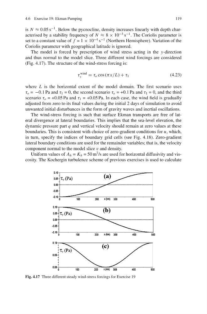
The model is forced by prescription of wind stress acting in the y-direction
and thus normal to the model slice. Three different wind forcings are considered
(Fig. 4.17). The structure of the wind-stress forcing is:
τ
wind
y
= τ o cos (π x/L) + τ 1
(4.23)
where L is the horizontal extent of the model domain. The first scenario uses
τ o = −0.1 Pa and τ 1 = 0, the second scenario τ o = +0.1 Pa and τ 1 = 0, and the third
scenario τ o = +0.05 Pa and τ 1 = +0.05 Pa. In each case, the wind field is gradually
adjusted from zero to its final values during the initial 2 days of simulation to avoid
unwanted initial disturbances in the form of gravity waves and inertial oscillations.
The wind-stress forcing is such that surface Ekman transports are free of lateral divergence at lateral boundaries. This implies that the sea-level elevation, the
dynamic pressure part q and vertical velocity should remain at zero values at these
boundaries. This is consistent with choice of zero-gradient conditions for u, which,
in turn, specify the indices of boundary grid cells (see Fig. 4.18). Zero-gradient
lateral boundary conditions are used for the remainder variables; that is, the velocity
component normal to the model slice v and density.
Uniform values of A h = K h = 50 m
2 /s are used for horizontal diffusivity and viscosity. The Kochergin turbulence scheme of previous exercises is used to calculate
Fig. 4.17 Three different steady wind-stress forcings for Exercise 19
119
is N ≈ 0.05 s
−1 . Below the pycnocline, density increases linearly with depth characterised by a stability frequency of N ≈ 8 × 10
−3 s
−1 . The Coriolis parameter is
set to a constant value of f = 1 × 10
−4 s
−1 (Northern Hemisphere). Variation of the
Coriolis parameter with geographical latitude is ignored.
The model is forced by prescription of wind stress acting in the y-direction
and thus normal to the model slice. Three different wind forcings are considered
(Fig. 4.17). The structure of the wind-stress forcing is:
τ
wind
y
= τ o cos (π x/L) + τ 1
(4.23)
where L is the horizontal extent of the model domain. The first scenario uses
τ o = −0.1 Pa and τ 1 = 0, the second scenario τ o = +0.1 Pa and τ 1 = 0, and the third
scenario τ o = +0.05 Pa and τ 1 = +0.05 Pa. In each case, the wind field is gradually
adjusted from zero to its final values during the initial 2 days of simulation to avoid
unwanted initial disturbances in the form of gravity waves and inertial oscillations.
The wind-stress forcing is such that surface Ekman transports are free of lateral divergence at lateral boundaries. This implies that the sea-level elevation, the
dynamic pressure part q and vertical velocity should remain at zero values at these
boundaries. This is consistent with choice of zero-gradient conditions for u, which,
in turn, specify the indices of boundary grid cells (see Fig. 4.18). Zero-gradient
lateral boundary conditions are used for the remainder variables; that is, the velocity
component normal to the model slice v and density.
Uniform values of A h = K h = 50 m
2 /s are used for horizontal diffusivity and viscosity. The Kochergin turbulence scheme of previous exercises is used to calculate
Fig. 4.17 Three different steady wind-stress forcings for Exercise 19