

4.3 Exercise 17: Tidal-Mixing Fronts
109
fronts) tend to become dynamically unstable and break up into mesoscale eddies
inducing vigorous lateral mixing across the front. This cannot be simulated with the
2.5d model.
4.3.4 Additional Study
Prognostic advection-diffusion equations for Eulerian tracer concentration fields are
added to the code to quantify the sources of water that make up the frontal zone. To
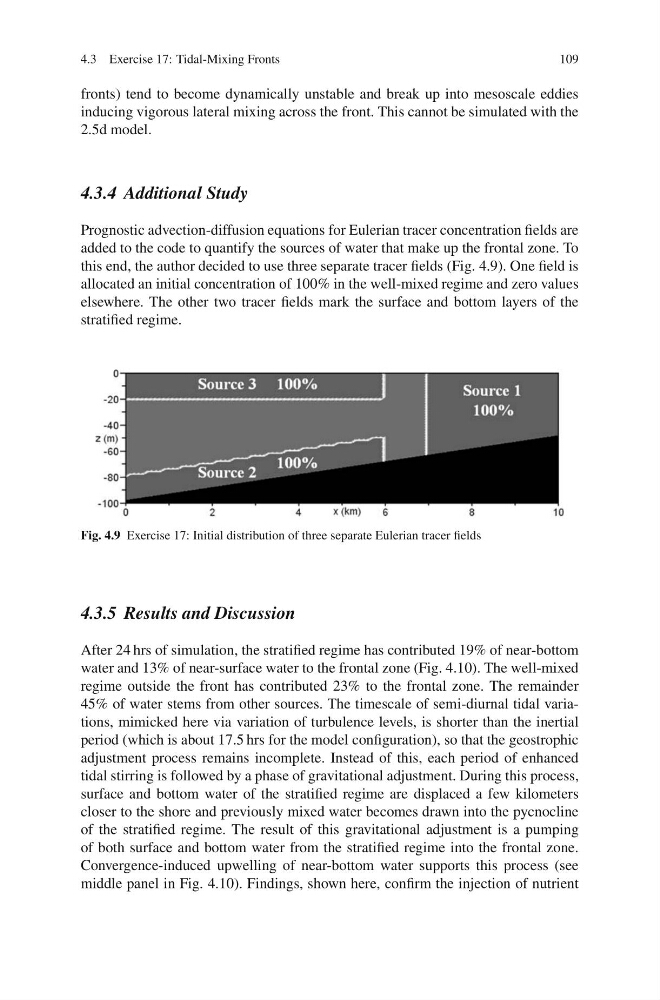
this end, the author decided to use three separate tracer fields (Fig. 4.9). One field is
allocated an initial concentration of 100% in the well-mixed regime and zero values
elsewhere. The other two tracer fields mark the surface and bottom layers of the
stratified regime.
Fig. 4.9 Exercise 17: Initial distribution of three separate Eulerian tracer fields
4.3.5 Results and Discussion
After 24 hrs of simulation, the stratified regime has contributed 19% of near-bottom
water and 13% of near-surface water to the frontal zone (Fig. 4.10). The well-mixed
regime outside the front has contributed 23% to the frontal zone. The remainder
45% of water stems from other sources. The timescale of semi-diurnal tidal variations, mimicked here via variation of turbulence levels, is shorter than the inertial
period (which is about 17.5 hrs for the model configuration), so that the geostrophic
adjustment process remains incomplete. Instead of this, each period of enhanced
tidal stirring is followed by a phase of gravitational adjustment. During this process,
surface and bottom water of the stratified regime are displaced a few kilometers
closer to the shore and previously mixed water becomes drawn into the pycnocline
of the stratified regime. The result of this gravitational adjustment is a pumping
of both surface and bottom water from the stratified regime into the frontal zone.
Convergence-induced upwelling of near-bottom water supports this process (see
middle panel in Fig. 4.10). Findings, shown here, confirm the injection of nutrient
109
fronts) tend to become dynamically unstable and break up into mesoscale eddies
inducing vigorous lateral mixing across the front. This cannot be simulated with the
2.5d model.
4.3.4 Additional Study
Prognostic advection-diffusion equations for Eulerian tracer concentration fields are
added to the code to quantify the sources of water that make up the frontal zone. To
this end, the author decided to use three separate tracer fields (Fig. 4.9). One field is
allocated an initial concentration of 100% in the well-mixed regime and zero values
elsewhere. The other two tracer fields mark the surface and bottom layers of the
stratified regime.
Fig. 4.9 Exercise 17: Initial distribution of three separate Eulerian tracer fields
4.3.5 Results and Discussion
After 24 hrs of simulation, the stratified regime has contributed 19% of near-bottom
water and 13% of near-surface water to the frontal zone (Fig. 4.10). The well-mixed
regime outside the front has contributed 23% to the frontal zone. The remainder
45% of water stems from other sources. The timescale of semi-diurnal tidal variations, mimicked here via variation of turbulence levels, is shorter than the inertial
period (which is about 17.5 hrs for the model configuration), so that the geostrophic
adjustment process remains incomplete. Instead of this, each period of enhanced
tidal stirring is followed by a phase of gravitational adjustment. During this process,
surface and bottom water of the stratified regime are displaced a few kilometers
closer to the shore and previously mixed water becomes drawn into the pycnocline
of the stratified regime. The result of this gravitational adjustment is a pumping
of both surface and bottom water from the stratified regime into the frontal zone.
Convergence-induced upwelling of near-bottom water supports this process (see
middle panel in Fig. 4.10). Findings, shown here, confirm the injection of nutrient