

88
3 Basics of Nonhydrostatic Modelling
Residence time is the time it takes for a virtual water parcel to escape from a given
area. Particle-tracking methods, using Lagrangian floats such as in Exercise 9, are
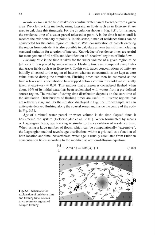
used to calculate this timescale. For the circulation shown in Fig. 3.51, for instance,
the residence time of a water parcel released at point A is the time it takes until it
reaches the exit boundary at point B. In this sense, a map of residence times can be
constructed for the entire region of interest. With consideration of parcels entering
the region from outside, it is also possible to calculate a mean transit time including
standard variation for a region of interest. Knowledge of residence times are useful
for management of oil spills and identification of “shadow” regions of little flow.
Flushing time is the time it takes for the water volume of a given region to be
(almost) fully replaced by ambient water. Flushing times are computed using Eulerian tracer fields such as in Exercise 9. To this end, tracer concentrations of unity are
initially allocated to the region of interest whereas concentrations are kept at zero
value outside during the simulation. Flushing times can then be estimated as the
time is takes until concentration has dropped below a certain threshold value usually
taken at exp (−π) ≈ 0.04. This implies that a region is considered flushed when
about 96% of its initial water has been replenished with waters from a pre-defined
source region. The resultant flushing time distribution depends on the start time of
the simulation. Distributions of flushing times are useful to illustrate regions that
are relatively stagnant. For the situation displayed in Fig. 3.51, for example, we can
anticipate delayed flushing along the coastal zones and inside the centre of the eddy
in Fig. 3.51.
Age of a virtual water parcel or water volume is the time elapsed since it
has entered the system (Deleersnijder et al., 2001). When formulated by means
of Lagrangian floats, age tracking is similar to the calculation of residence time.
When using a large number of floats, which can be computationally “expensive”,
the Lagrangian method reveals age distributions within a grid cell as a function of
both location and time. Nevertheless, water age is usually calculated from Eulerian
concentration fields according to the modified advection-diffusion equation:
∂ A
∂t
+ Adv(A) = Diff(A) + 1
(3.82)
Fig. 3.51 Schematic for
explanation of residence time
and flushing time. Shaded
areas represent regions of
delayed flushing
3 Basics of Nonhydrostatic Modelling
Residence time is the time it takes for a virtual water parcel to escape from a given
area. Particle-tracking methods, using Lagrangian floats such as in Exercise 9, are
used to calculate this timescale. For the circulation shown in Fig. 3.51, for instance,
the residence time of a water parcel released at point A is the time it takes until it
reaches the exit boundary at point B. In this sense, a map of residence times can be
constructed for the entire region of interest. With consideration of parcels entering
the region from outside, it is also possible to calculate a mean transit time including
standard variation for a region of interest. Knowledge of residence times are useful
for management of oil spills and identification of “shadow” regions of little flow.
Flushing time is the time it takes for the water volume of a given region to be
(almost) fully replaced by ambient water. Flushing times are computed using Eulerian tracer fields such as in Exercise 9. To this end, tracer concentrations of unity are
initially allocated to the region of interest whereas concentrations are kept at zero
value outside during the simulation. Flushing times can then be estimated as the
time is takes until concentration has dropped below a certain threshold value usually
taken at exp (−π) ≈ 0.04. This implies that a region is considered flushed when
about 96% of its initial water has been replenished with waters from a pre-defined
source region. The resultant flushing time distribution depends on the start time of
the simulation. Distributions of flushing times are useful to illustrate regions that
are relatively stagnant. For the situation displayed in Fig. 3.51, for example, we can
anticipate delayed flushing along the coastal zones and inside the centre of the eddy
in Fig. 3.51.
Age of a virtual water parcel or water volume is the time elapsed since it
has entered the system (Deleersnijder et al., 2001). When formulated by means
of Lagrangian floats, age tracking is similar to the calculation of residence time.
When using a large number of floats, which can be computationally “expensive”,
the Lagrangian method reveals age distributions within a grid cell as a function of
both location and time. Nevertheless, water age is usually calculated from Eulerian
concentration fields according to the modified advection-diffusion equation:
∂ A
∂t
+ Adv(A) = Diff(A) + 1
(3.82)
Fig. 3.51 Schematic for
explanation of residence time
and flushing time. Shaded
areas represent regions of
delayed flushing