

76
4 Long Waves in a Channel
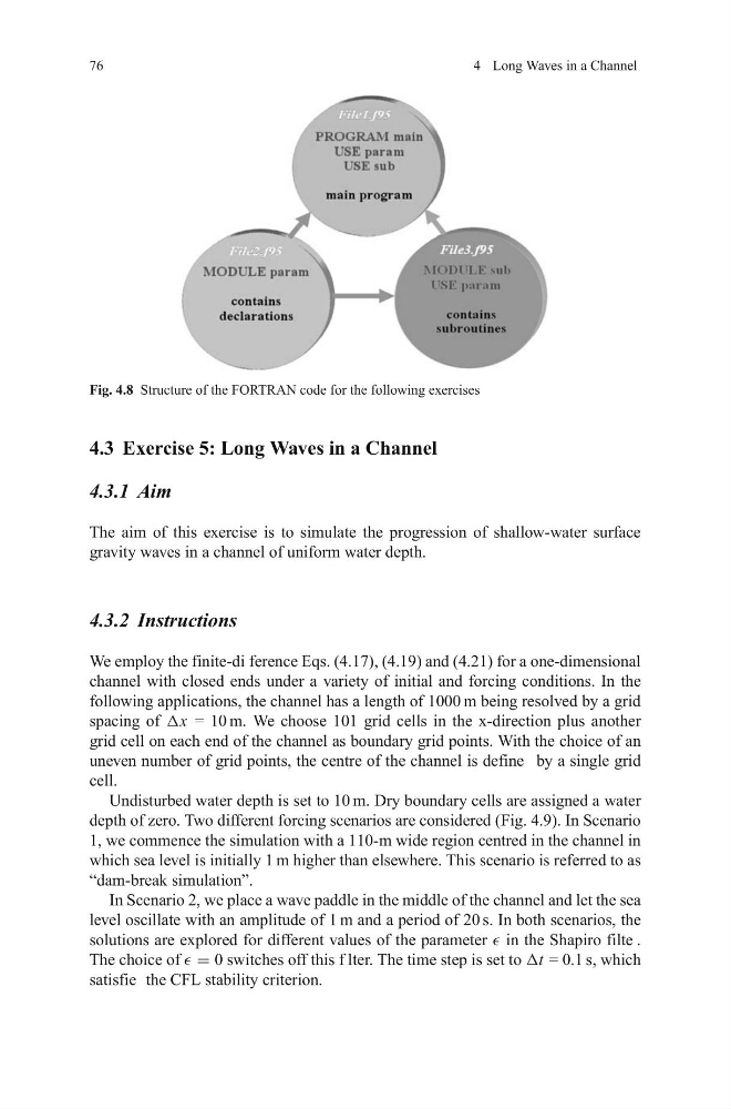
Fig. 4.8 Structure of the FORTRAN code for the following exercises
4.3 Exercise 5: Long Waves in a Channel
4.3.1 Aim
The aim of this exercise is to simulate the progression of shallow-water surface
gravity waves in a channel of uniform water depth.
4.3.2 Instructions
We employ the finite-di ference Eqs. (4.17), (4.19) and (4.21) for a one-dimensional
channel with closed ends under a variety of initial and forcing conditions. In the
following applications, the channel has a length of 1000 m being resolved by a grid
spacing of Δx = 10 m. We choose 101 grid cells in the x-direction plus another
grid cell on each end of the channel as boundary grid points. With the choice of an
uneven number of grid points, the centre of the channel is define by a single grid
cell.
Undisturbed water depth is set to 10 m. Dry boundary cells are assigned a water
depth of zero. Two different forcing scenarios are considered (Fig. 4.9). In Scenario
1, we commence the simulation with a 110-m wide region centred in the channel in
which sea level is initially 1 m higher than elsewhere. This scenario is referred to as
“dam-break simulation”.
In Scenario 2, we place a wave paddle in the middle of the channel and let the sea
level oscillate with an amplitude of 1 m and a period of 20 s. In both scenarios, the
solutions are explored for different values of the parameter in the Shapiro filte .
The choice of = 0 switches off this f lter. The time step is set to Δt = 0.1 s, which
satisfie the CFL stability criterion.
4 Long Waves in a Channel
Fig. 4.8 Structure of the FORTRAN code for the following exercises
4.3 Exercise 5: Long Waves in a Channel
4.3.1 Aim
The aim of this exercise is to simulate the progression of shallow-water surface
gravity waves in a channel of uniform water depth.
4.3.2 Instructions
We employ the finite-di ference Eqs. (4.17), (4.19) and (4.21) for a one-dimensional
channel with closed ends under a variety of initial and forcing conditions. In the
following applications, the channel has a length of 1000 m being resolved by a grid
spacing of Δx = 10 m. We choose 101 grid cells in the x-direction plus another
grid cell on each end of the channel as boundary grid points. With the choice of an
uneven number of grid points, the centre of the channel is define by a single grid
cell.
Undisturbed water depth is set to 10 m. Dry boundary cells are assigned a water
depth of zero. Two different forcing scenarios are considered (Fig. 4.9). In Scenario
1, we commence the simulation with a 110-m wide region centred in the channel in
which sea level is initially 1 m higher than elsewhere. This scenario is referred to as
“dam-break simulation”.
In Scenario 2, we place a wave paddle in the middle of the channel and let the sea
level oscillate with an amplitude of 1 m and a period of 20 s. In both scenarios, the
solutions are explored for different values of the parameter in the Shapiro filte .
The choice of = 0 switches off this f lter. The time step is set to Δt = 0.1 s, which
satisfie the CFL stability criterion.